Date: This Edition: September 14, 2005, 14:03:21; Revision History: Section 11.
Start by downloading either the file KnotTheory.tar.gz (1051Kb) or the file KnotTheory.zip (1132Kb), and unpack either one. This will create a subdirectory KnotTheory/ in your current working directory. This done, no installation is required (though you may wish to check out ``Further Data Files'' below). Start Mathematica and you're ready to go:
In[1]:= |
<< KnotTheory` |
Loading KnotTheory` (version of September 14, 2005, 13:37:36)... | |
Let us check that everything is working well:
In[2]:= | Alexander[Knot[6, 2]][t] |
Out[2]= | -2 3 2
-3 - t + - + 3 t - t
t |
|
In[3]:= ?KnotTheoryVersion
In[4]:= ?KnotTheoryVersionString
In[5]:= ?KnotTheoryWelcomeMessage
|
Thus on the day this manual page was last changed, we had:
In[6]:= | {KnotTheoryVersion[], KnotTheoryVersionString[]} |
Out[6]= | {{2005, 9, 14, 13, 37, 36}, September 14, 2005, 13:37:36} |
|
In[7]:= ?KnotTheoryDirectory
|
Thus with my setup,
In[8]:= | KnotTheoryDirectory[] |
Out[8]= | ./KnotTheory |
KnotTheoryDirectory may not work under some operating systems/environments. Please let me know if you encounter any difficulties.
Notes.
KnotTheory` comes loaded with some knot tables; currently, the Rolfsen table of prime knots with up to 10 crossings [Ro], the Hoste-Thistlethwaite tables of prime knots with up to 16 crossings and the Thistlethwaite table of prime links with up to 11 crossings (Section 10.2):
|
In[2]:= ?Knot
In[3]:= ?Link
|
![\begin{figure}\centering {
\includegraphics[height=2cm]{figs/6.1.eps}
\qquad\i...
...{figs/9.46.eps}
\qquad\includegraphics[height=2cm]{figs/L6a4.ps}
}
\end{figure}](img10.gif) |
Thus, for example, let us verify that the knots
![]() and
and
![]() have the same Alexander
polynomial:
have the same Alexander
polynomial:
In[4]:= | Alexander[Knot[6, 1]][t] |
Out[4]= | 2
5 - - - 2 t
t |
In[5]:= | Alexander[Knot[9, 46]][t] |
Out[5]= | 2
5 - - - 2 t
t |
We can also check that the Borromean rings, L6a4 in the Thistlethwaite table, is a 3-component link:
In[6]:= | Length[Skeleton[Link[6, Alternating, 4]]] |
Out[6]= | 3 |
|
In[7]:= ?AllKnots
In[8]:= ?AllLinks
|
Thus at the moment there are 802 knots and 1424 links known to KnotTheory`:
In[9]:= | Length /@ {AllKnots[], AllLinks[]} |
Out[9]= | {802, 1424} |
Note though that if you have also loaded the further files DTCodes4Knots12To16.tar.gz (8252Kb) or DTCodes4Knots12To16.zip (8244Kb), the contents of AllKnots[] does not change but higher knots in the Hoste-Thistlethwaite enumeration become available:
In[10]:= | Show[DrawPD[Knot[13, NonAlternating, 5016], {Gap -> 0.025}]] |
 | |
Out[10]= | -Graphics- |
(Shumakovitch had noticed that this nice knot has interesting Khovanov homology; see [Sh, Section A.4]).
In addition to the tables, KnotTheory` also knows about torus knots:
|
In[11]:= ?TorusKnot
|
For example, the torus knots T(5,3) and
T(3,5) have different presentations with different numbers of crossings,
but they are in fact isotopic, and hence they have the same invariants
(and in particular the same type 3 Vassiliev invariant ![]() ):
):
In[12]:= | Crossings /@ {TorusKnot[5,3], TorusKnot[3, 5]} |
Out[12]= | {10, 12} |
In[13]:= | Vassiliev[3] /@ {TorusKnot[5,3], TorusKnot[3, 5]} |
Out[13]= | {20, 20} |
KnotTheory` knows how to plot torus knots; see Section 8.1.
For KnotTheory`, we present every knot or link diagram (every
Planar Diagram or just PD) by labeling its edges (with natural
numbers, 1,...,n, and with increasing labels as we go around each
component) and by a list crossings presented as symbols ![]() where
where ![]() ,
, ![]() ,
, ![]() and
and ![]() are the labels of the edges around that
crossing, starting from the incoming lower edge
and proceeding counterclockwise. Thus for example, the PD presentation
of the knot in Figure 2 is:
are the labels of the edges around that
crossing, starting from the incoming lower edge
and proceeding counterclockwise. Thus for example, the PD presentation
of the knot in Figure 2 is:
|
In[2]:= ?PD
In[3]:= PD::about
In[4]:= ?X
|
Thus, for example, let us compute the determinant of the above knot:
In[5]:= | K = PD[ X[1,9,2,8], X[3,10,4,11], X[5,3,6,2], X[7,1,8,12], X[9,4,10,5], X[11,7,12,6] ]; |
In[6]:= | Alexander[K][-1] |
Out[6]= | -11 |
|
In[7]:= ?Xp
In[8]:= ?Xm
In[9]:= ?P
|
For example, we could add an extra ``point'' on the Miller Institute knot, splitting edge 12 into two pieces, labeled 12 and 13:
In[10]:= | K1 = PD[ X[1,9,2,8], X[3,10,4,11], X[5,3,6,2], X[7,1,8,13], X[9,4,10,5], X[11,7,12,6], P[12,13] ]; |
At the moment, many of our routines do not know to ignore such ``extra points''. But some do:
In[11]:= | Jones[K][q] == Jones[K1][q] |
Out[11]= | True |
|
In[12]:= ?Loop
|
Hence we can verify that the A2 invariant of the unknot is
![]() :
:
In[13]:= | A2Invariant[Loop[1]][q] |
Out[13]= | -2 2 1 + q + q |
The Gauss Code of an ![]() -crossing
knot or link
-crossing
knot or link ![]() is obtained as follows:
is obtained as follows:
The resulting list of signed integers (in the case of a knot) or list of
lists of signed integers (in the case of a link) is called the Gauss
Code of ![]() . KnotTheory` has some rudimentary support for Gauss
codes:
. KnotTheory` has some rudimentary support for Gauss
codes:
|
In[2]:= ?GaussCode
|
Thus for example, the Gauss codes for the trefoil knot and the Borromean link are:
In[3]:= | GaussCode /@ {Knot[3, 1], Link[6, Alternating, 4]} |
Out[3]= | {GaussCode[-1, 3, -2, 1, -3, 2],
> GaussCode[{1, -6, 5, -3}, {4, -1, 2, -5}, {6, -4, 3, -2}]} |
Ralph Furmaniak, working under the guidance of Stuart Rankin and Ortho Flint at the University of Western Ontario, wrote a web-based server called ``Knotilus'' that takes Gauss codes and outputs pictures of the desired knots and links in several standard image formats.
|
In[4]:= ?KnotilusURL
|
Thus,
In[5]:= | KnotilusURL /@ {Knot[3, 1], Link[6, Alternating, 4]} |
Out[5]= | {http://srankin.math.uwo.ca/cgi-bin/retrieve.cgi/-1,3,-2,1,-3,2/goTop.html,
> http://srankin.math.uwo.ca/cgi-bin/retrieve.cgi/1,-6,5,-3:4,-1,2,-5:6,-4,\
> 3,-2/goTop.html} |
Click to get there! http://srankin.math.uwo.ca/cgi-bin/retrieve.cgi/-1,3,-2,1,-3,2/goTop.html and http://srankin.math.uwo.ca/cgi-bin/retrieve.cgi/1,-6,5,-3:4,-1,2,-5:6,-4,3,-2/goTop.html.
The DT Code (``DT'' after
Clifford
Hugh Dowker and Morwen
Thistlethwaite) of a knot ![]() is obtained as follows:
is obtained as follows:
KnotTheory` has some rudimentary support for DT codes:
|
In[2]:= ?DTCode
|
Thus for example, the DT codes for the last 9 crossing alternating knot
![]() and the first 9 crossing non
alternating knot
and the first 9 crossing non
alternating knot ![]() are:
are:
In[3]:= | dts = DTCode /@ {Knot[9, 41], Knot[9, 42]} |
Out[3]= | {DTCode[6, 10, 14, 12, 16, 2, 18, 4, 8],
> DTCode[4, 8, 10, -14, 2, -16, -18, -6, -12]} |
(The DT code of an alternating knot is always a sequence of positive numbers but the DT code of a non alternating knot contains both signs.)
DT codes and Gauss codes carry the same information and are easily convertible:
In[4]:= | gcs = GaussCode /@ dts |
Out[4]= | {GaussCode[1, -6, 2, -8, 3, -1, 4, -9, 5, -2, 6, -4, 7, -3, 8, -5, 9, -7],
> GaussCode[1, -5, 2, -1, 3, 8, -4, -2, 5, -3, -6, 9, -7, 4, -8, 6, -9, 7]} |
In[5]:= | DTCode /@ gcs |
Out[5]= | {DTCode[6, 10, 14, 12, 16, 2, 18, 4, 8],
> DTCode[4, 8, 10, -14, 2, -16, -18, -6, -12]} |
Conversion between DT codes and/or Gauss codes and PD codes is more complicated; the harder side, going from DT/Gauss to PD, was written by Siddarth Sankaran at the University of Toronto:
In[6]:= | PD[DTCode[4, 6, 2]] |
Out[6]= | PD[X[4, 2, 5, 1], X[6, 4, 1, 3], X[2, 6, 3, 5]] |
Every knot and every link is the closure of a braid. KnotTheory` can also represent knots and links as braid closures:
|
In[2]:= ?BR
In[3]:= BR::about
In[4]:= ?Mirror
|
Thus for example,
In[5]:= | br1 = BR[2, {-1, -1, -1}]; |
In[6]:= | PD[br1, q] |
Out[6]= | PD[BR[2, {-1, -1, -1}], q] |
In[7]:= | Jones[br1][q] |
Out[7]= | -4 -3 1
-q + q + -
q |
In[8]:= | Mirror[br1] |
Out[8]= | BR[2, {1, 1, 1}] |
KnotTheory` has the braid representatives of some knots and links pre-loaded. Thus for example,
In[9]:= | BR[TorusKnot[5, 4]] |
Out[9]= | BR[4, {1, 2, 3, 1, 2, 3, 1, 2, 3, 1, 2, 3, 1, 2, 3}] |
The minimum braid representative of a given knot is a braid
representative for that knot which has a minimal number of braid
crossings and within those braid representatives with a minimal number
of braid crossings, it has a minimal number of strands (full details
are in Gittings' [Gi]). Thomas Gittings kindly
provided us the minimum braid representatives for all knots with up to 10
crossings. Thus for example, the minimum braid representative for the knot
![]() has length (number of crossings)
13 and width (number of strands, also see
Section 7.1) 6:
has length (number of crossings)
13 and width (number of strands, also see
Section 7.1) 6:
In[10]:= | br2 = BR[Knot[10, 1]] |
Out[10]= | BR[6, {-1, -1, -2, 1, -2, -3, 2, -3, -4, 3, 5, -4, 5}] |
In[11]:= | Show[BraidPlot[CollapseBraid[br2]]] |
 | |
Out[11]= | -Graphics- |
(Check Section 5.2 for information about the command BraidPlot and the related command CollapseBraid.)
My summer student Emily Redelmeier is in the process of writing a program that uses circle packing to draw an arbitrary object given as a PD as in Section 4.1. At the moment her program is still slow, limited and sometimes buggy, but it is already quite useful, as the following lines show:
|
In[2]:= ?DrawPD
In[3]:= DrawPD::about
|
Thus, for example, here's the torus knot T(4,3):
In[4]:= | Show[DrawPD[TorusKnot[4, 3]]] |
 | |
Out[4]= | -Graphics- |
One problem we currently have is that crossings come out at non-uniform sizes, hence in the picture below you may need magnifying glasses to decide who's over and who's under:
In[5]:= | MillettUnknot = PD[ X[1,10,2,11], X[9,2,10,3], X[3,7,4,6], X[15,5,16,4], X[5,17,6,16], X[7,14,8,15], X[8,18,9,17], X[11,18,12,19], X[19,12,20,13], X[13,20,14,1] ]; |
In[6]:= | Show[DrawPD[MillettUnknot]] |
 | |
Out[6]= | -Graphics- |
In such a situation, the option Gap is sometimes handy:
In[7]:= | Show[DrawPD[MillettUnknot, {Gap -> 0.03}]] |
 | |
Out[7]= | -Graphics- |
 |
 |
But now every ingredient of the original knot (every arc, crossing and
face) has a disk in the plane in which it can be cleanly drawn and
clashes are guaranteed not to occur. Furthermore, knowing the precise
coordinates of all the tangency points allows us to represent each
ingredient by some nice smooth arcs that meet smoothly. The result is
the right half of the picture above. Removing all the circles, what
remains is the desired clean planar picture of
![]() .
.
|
In[2]:= ?BraidPlot
In[3]:= Options[BraidPlot]
|
Thus for example,
In[4]:= | br = BR[5, {{1,3}, {-2,-4}, {1, 3}}] |
Out[4]= | BR[5, {{1, 3}, {-2, -4}, {1, 3}}] |
In[5]:= | Show[BraidPlot[br]] |
 | |
Out[5]= | -Graphics- |
The Mode option to BraidPlot defaults to "Graphics",
which produces output as above. An alternative is setting
Mode -> "HTML", which produces an HTML <table> that can be
readily inserted into HTML documents:
In[6]:= | BraidPlot[br, Mode -> "HTML"] |
Out[6]= | <table cellspacing=0 cellpadding=0 border=0> <tr><td><img src=1.gif><img src=0.gif><img src=1.gif></td></tr> <tr><td><img src=2.gif><img src=3.gif><img src=2.gif></td></tr> <tr><td><img src=1.gif><img src=4.gif><img src=1.gif></td></tr> <tr><td><img src=2.gif><img src=3.gif><img src=2.gif></td></tr> <tr><td><img src=0.gif><img src=4.gif><img src=0.gif></td></tr> </table> |
The table produced contains an array of image inclusions that together draws the braid using 5 fundamental building blocks: a horizontal ``unbraided'' line (0.gif above), the upper and lower halves of an overcrossing (1.gif and 2.gif above) and the upper and lower halves of an underfcrossing (3.gif and 4.gif above).
Assuming 0.gif through 4.gif are
 ,
,  ,
,  ,
,
 and
and  ,
the above table is rendered as follows:
,
the above table is rendered as follows:
|
|
|
|
|
The meaning of the Images option to BraidPlot should be clear from reading its default definition:
In[7]:= | Images /. Options[BraidPlot] |
Out[7]= | {0.gif, 1.gif, 2.gif, 3.gif, 4.gif} |
The HTMLOpts option to BraidPlot allows to insert options
within the HTML <img> tags. Thus
In[8]:= | BraidPlot[ BR[2, {1, 1}], Mode -> "HTML", HTMLOpts -> "border=1" ] |
Out[8]= | <table cellspacing=0 cellpadding=0 border=0> <tr><td><img border=1 src=1.gif><img border=1 src=1.gif></td></tr> <tr><td><img border=1 src=2.gif><img border=1 src=2.gif></td></tr> </table> |
the above table is rendered as follows:
|
|
|
In[9]:= ?CollapseBraid
|
Thus compare the plots of br1 and br2 below:
In[10]:= | br1 = BR[TorusKnot[5, 4]] |
Out[10]= | BR[4, {1, 2, 3, 1, 2, 3, 1, 2, 3, 1, 2, 3, 1, 2, 3}] |
In[11]:= | Show[BraidPlot[br1]] |
 | |
Out[11]= | -Graphics- |
In[12]:= | br2 = CollapseBraid[BR[TorusKnot[5, 4]]] |
Out[12]= | BR[4, {{1}, {2}, {3, 1}, {2}, {3, 1}, {2}, {3, 1}, {2}, {3, 1}, {2}, {3}}] |
In[13]:= | Show[BraidPlot[br2]] |
 | |
Out[13]= | -Graphics- |
|
In[2]:= ?Crossings
In[3]:= ?PositiveCrossings
In[4]:= ?NegativeCrossings
|
Thus here's one tautology and one easy example:
In[5]:= | Crossings /@ {Knot[0, 1], TorusKnot[11,10]} |
Out[5]= | {0, 99} |
And another easy example:
In[6]:= | K=Knot[6, 2]; {PositiveCrossings[K], NegativeCrossings[K]} |
Out[6]= | {2, 4} |
|
In[7]:= ?PositiveQ
In[8]:= ?NegativeQ
|
For example,
In[9]:= | PositiveQ /@ {X[1,3,2,4], X[1,4,2,3], Xp[1,3,2,4], Xp[1,4,2,3]} |
Out[9]= | {False, True, True, True} |
|
In[10]:= ?ConnectedSum
|
The connected sum
![]() of the knot
of the knot
![]() with itself has 8 crossings
(unsurprisingly):
with itself has 8 crossings
(unsurprisingly):
In[11]:= | K = ConnectedSum[Knot[4,1], Knot[4,1]] |
Out[11]= | ConnectedSum[Knot[4, 1], Knot[4, 1]] |
In[12]:= | Crossings[K] |
Out[12]= | 8 |
It is also nice to know that, as expected, the Jones polynomial of ![]() is
the square of the Jones polynomial of
is
the square of the Jones polynomial of ![]() :
:
In[13]:= | Jones[K][q] == Expand[Jones[Knot[4,1]][q]^2] |
Out[13]= | True |
It is less nice to know that the Jones polynomial cannot tell ![]() apart
from the knot
apart
from the knot ![]() :
:
In[14]:= | Jones[K][q] == Jones[Knot[8,9]][q] |
Out[14]= | True |
But ![]() isn't equivalent to
isn't equivalent to ![]() ;
indeed, their Alexander polynomials are different:
;
indeed, their Alexander polynomials are different:
In[15]:= | {Alexander[K][t], Alexander[Knot[8,9]][t]} |
Out[15]= | -2 6 2 -3 3 5 2 3
{11 + t - - - 6 t + t , 7 - t + -- - - - 5 t + 3 t - t }
t 2 t
t |
The braid length of a knot or a link ![]() is the smallest number of
crossings in a braid whose closure is
is the smallest number of
crossings in a braid whose closure is ![]() . KnotTheory` has some braid
lengths preloaded:
. KnotTheory` has some braid
lengths preloaded:
|
In[2]:= ?BraidLength
|
Note that the braid length of ![]() is simply the length of the minimum
braid representing
is simply the length of the minimum
braid representing ![]() (see Section 4.4):
(see Section 4.4):
In[3]:= | K = Knot[9, 49]; {BraidLength[K], Crossings[BR[K]]} |
Out[3]= | {11, 11} |
The braid index of a knot or a link ![]() is the smallest number of
strands in a braid whose closure is
is the smallest number of
strands in a braid whose closure is ![]() . KnotTheory` has some braid
indices preloaded:
. KnotTheory` has some braid
indices preloaded:
|
In[4]:= ?BraidIndex
In[5]:= BraidIndex::about
|
Of the 250 knots with up to 10 crossings, only
![]() has braid index smaller than
the width of its minimum braid:
has braid index smaller than
the width of its minimum braid:
In[6]:= | K = Knot[10, 136]; {BraidIndex[K], First@BR[K]} |
Out[6]= | {4, 5} |
In[7]:= | Show[BraidPlot[BR[K]]] |
 | |
Out[7]= | -Graphics- |
|
In[2]:= ?SymmetryType
In[3]:= SymmetryType::about
|
The unknotting number of a knot ![]() is the minimal number of crossing
changes needed in order to unknot
is the minimal number of crossing
changes needed in order to unknot ![]() .
.
|
In[4]:= ?UnknottingNumber
In[5]:= UnknottingNumber::about
|
Of the 512 knots whose unknotting number is known to KnotTheory`, 197 have unknotting number 1, 247 have unknotting number 2, 54 have unknotting number 3, 12 have unknotting number 4 and 1 has unknotting number 5:
In[6]:= | Plus @@ u /@ Cases[UnknottingNumber /@ AllKnots[], _Integer] |
Out[6]= | u[0] + 197 u[1] + 247 u[2] + 54 u[3] + 12 u[4] + u[5] |
There are 4 knots with up to 9 crossings whose unknotting number is unknown:
In[7]:= | Select[AllKnots[], Crossings[#] <= 9 && Head[UnknottingNumber[#]] === List &] |
Out[7]= | {Knot[9, 10], Knot[9, 13], Knot[9, 35], Knot[9, 38]} |
|
In[8]:= ?ThreeGenus
In[9]:= ThreeGenus::about
|
The bridge index of a knot ![]() is the minimal number of local maxima (or
local minima) in a generic smooth embedding of
is the minimal number of local maxima (or
local minima) in a generic smooth embedding of ![]() in
in
![]() .
.
|
In[10]:= ?BridgeIndex
In[11]:= BridgeIndex::about
|
An often studied class of knots is the class of 2-bridge knots, knots whose bridge index is 2. Of the 49 9-crossings knots, 24 are 2-bridge:
In[12]:= | Select[AllKnots[], Crossings[#] == 9 && BridgeIndex[#] == 2 &] |
Out[12]= | {Knot[9, 1], Knot[9, 2], Knot[9, 3], Knot[9, 4], Knot[9, 5], Knot[9, 6],
> Knot[9, 7], Knot[9, 8], Knot[9, 9], Knot[9, 10], Knot[9, 11],
> Knot[9, 12], Knot[9, 13], Knot[9, 14], Knot[9, 15], Knot[9, 17],
> Knot[9, 18], Knot[9, 19], Knot[9, 20], Knot[9, 21], Knot[9, 23],
> Knot[9, 26], Knot[9, 27], Knot[9, 31]} |
The super bridge index of a knot ![]() is the minimal number, in a
generic smooth embedding of
is the minimal number, in a
generic smooth embedding of ![]() in
in
![]() , of the maximal number of local
maxima (or local minima) in a rigid rotation of that projection.
, of the maximal number of local
maxima (or local minima) in a rigid rotation of that projection.
|
In[13]:= ?SuperBridgeIndex
In[14]:= SuperBridgeIndex::about
|
|
In[15]:= ?NakanishiIndex
In[16]:= NakanishiIndex::about
|
In[17]:= | Profile[K_] := Profile[ SymmetryType[K], UnknottingNumber[K], ThreeGenus[K] BridgeIndex[K], SuperBridgeIndex[K], NakanishiIndex[K] ] |
In[18]:= | Profile[Knot[9,24]] |
Out[18]= | Profile[Reversible, 1, 9, {4, 6}, 1] |
In[19]:= | Ks = Select[ AllKnots[], (Crossings[#] == 9 && Profile[#]==Profile[Knot[9,24]])& ] |
Out[19]= | {Knot[9, 24], Knot[9, 28], Knot[9, 30], Knot[9, 34]} |
In[20]:= | Alexander[#][t]& /@ Ks |
Out[20]= | -3 5 10 2 3
{13 - t + -- - -- - 10 t + 5 t - t ,
2 t
t
-3 5 12 2 3
> -15 + t - -- + -- + 12 t - 5 t + t ,
2 t
t
-3 5 12 2 3
> 17 - t + -- - -- - 12 t + 5 t - t ,
2 t
t
-3 6 16 2 3
> 23 - t + -- - -- - 16 t + 6 t - t }
2 t
t |
|
In[2]:= ?Alexander
In[3]:= Alexander::about
In[4]:= ?Conway
|
The Alexander polynomial ![]() and the Conway polynomial
and the Conway polynomial ![]() of a
knot
of a
knot ![]() always satisfy
always satisfy
![]() . Let us verify
this relation for the knot
. Let us verify
this relation for the knot ![]() :
:
In[5]:= | alex = Alexander[Knot[8, 18]][t] |
Out[5]= | -3 5 10 2 3
13 - t + -- - -- - 10 t + 5 t - t
2 t
t |
In[6]:= | Expand[Conway[Knot[8, 18]][Sqrt[t] - 1/Sqrt[t]]] |
Out[6]= | -3 5 10 2 3
13 - t + -- - -- - 10 t + 5 t - t
2 t
t |
The determinant of a knot ![]() is
is
![]() . Hence for
. Hence for
![]() it is
it is
In[7]:= | Abs[alex /. t -> -1] |
Out[7]= | 45 |
Alternatively (see Section 7.4):
In[8]:= | KnotDet[Knot[8, 18]] |
Out[8]= | 45 |
![]() , the (standardly normalized) type 2 Vassiliev invariant of
a knot
, the (standardly normalized) type 2 Vassiliev invariant of
a knot ![]() is the coefficient of
is the coefficient of ![]() in its Conway polynomial
in its Conway polynomial
In[9]:= | Coefficient[Conway[Knot[8, 18]][z], z^2] |
Out[9]= | 1 |
Alternatively (see Section 7.10),
In[10]:= | Vassiliev[2][Knot[8, 18]] |
Out[10]= | 0 |
Sometimes two knots have the same Alexander polynomial but different
Alexander ideals. An example is the pair
K11a99 and
K11a277. They have the same Alexander
polynomial, but the second Alexander ideal of the first knot is the whole
ring
![]() while the second Alexander ideal of the second knot is the
smaller ideal generated by
while the second Alexander ideal of the second knot is the
smaller ideal generated by ![]() and by
and by ![]() :
:
In[11]:= | {K1, K2} = {Knot[11, Alternating, 99], Knot[11, Alternating, 277]}; |
In[12]:= | Alexander[K1] == Alexander[K2] |
Out[12]= | True |
In[13]:= | Alexander[K1, 2][t] |
Out[13]= | {1} |
In[14]:= | Alexander[K2, 2][t] |
Out[14]= | {3, 1 + t} |
Finally, the Alexander polynomial attains 551 values on the 802 knots known to KnotTheory`:
In[15]:= | Length /@ {Union[Alexander[#]& /@ AllKnots[]], AllKnots[]} |
Out[15]= | {551, 802} |
|
In[2]:= ?KnotDet
In[3]:= ?KnotSignature
|
Thus, for example, the knots ![]() and
and ![]() have the same
determinant (and even the same Alexander and Jones polynomials), but
different signatures:
have the same
determinant (and even the same Alexander and Jones polynomials), but
different signatures:
In[4]:= | KnotDet /@ {Knot[5, 1], Knot[10, 132]} |
Out[4]= | {5, 5} |
In[5]:= | {
Equal @@ (Jones[#][q]& /@ {Knot[5, 1], Knot[10, 132]}),
Equal @@ (Alexander[#][t]& /@ {Knot[5, 1], Knot[10, 132]})
} |
Out[5]= | {True, True} |
In[6]:= | KnotSignature /@ {Knot[5, 1], Knot[10, 132]} |
Out[6]= | {-4, 0} |
|
In[2]:= ?Jones
|
In Section 3 we checked that the knots
![]() and
and
![]() have the same Alexander
polynomial. Their Jones polynomials are different, though:
have the same Alexander
polynomial. Their Jones polynomials are different, though:
In[3]:= | Jones[Knot[6, 1]][q] |
Out[3]= | -4 -3 -2 2 2
2 + q - q + q - - - q + q
q |
In[4]:= | Jones[Knot[9, 46]][q] |
Out[4]= | -6 -5 -4 2 -2 1
2 + q - q + q - -- + q - -
3 q
q |
The Jones polynomial attains 2110 values on the 2226 knots and links known to KnotTheory`:
In[5]:= | all = Join[AllKnots[], AllLinks[]]; |
In[6]:= | Length /@ {Union[Jones[#][q]& /@ all], all} |
Out[6]= | {2110, 2226} |
The Jones polynomial is so simple to compute using Mathematica that it's
worthwhile pause and see how this is done, even for readers with
limited prior programming experience. First, recall (say
from [Ka1]) the
definition of the Jones polynomial using the Kauffman bracket
![]() :
:
Just for concreteness, let us start by fixing ![]() to be the trefoil
knot (see Figure 6):
to be the trefoil
knot (see Figure 6):
In[7]:= | L = PD[Knot[3, 1]] |
Out[7]= | PD[X[1, 4, 2, 5], X[3, 6, 4, 1], X[5, 2, 6, 3]] |
Our first task is to perform the replacement
![]() on all crossings of
on all crossings of
![]() . By our conventions (see Section 4.1) the edges
around a crossing
. By our conventions (see Section 4.1) the edges
around a crossing ![]() are labeled
are labeled ![]() ,
, ![]() ,
, ![]() and
and ![]() :
:
![]() . Labeling
. Labeling
![]() and
and
![]() in the same way,
in the same way,
![]() and
and
![]() , we are lead to the symbolic
replacement rule
, we are lead to the symbolic
replacement rule
![]() . Let us apply
this rule to
. Let us apply
this rule to ![]() , switch to a multiplicative notation and expand:
, switch to a multiplicative notation and expand:
In[8]:= | t1 = L /. X[a_,b_,c_,d_] :> A P[a,d] P[b,c] + B P[a,b] P[c,d] |
Out[8]= | PD[A P[1, 5] P[2, 4] + B P[1, 4] P[2, 5], > B P[1, 4] P[3, 6] + A P[1, 3] P[4, 6], > A P[2, 6] P[3, 5] + B P[2, 5] P[3, 6]] |
In[9]:= | t2 = Expand[Times @@ t1] |
Out[9]= | 2
A B P[1, 4] P[1, 5] P[2, 4] P[2, 6] P[3, 5] P[3, 6] +
2 2
> A B P[1, 4] P[2, 5] P[2, 6] P[3, 5] P[3, 6] +
2 2
> A B P[1, 4] P[1, 5] P[2, 4] P[2, 5] P[3, 6] +
3 2 2 2
> B P[1, 4] P[2, 5] P[3, 6] +
3
> A P[1, 3] P[1, 5] P[2, 4] P[2, 6] P[3, 5] P[4, 6] +
2
> A B P[1, 3] P[1, 4] P[2, 5] P[2, 6] P[3, 5] P[4, 6] +
2
> A B P[1, 3] P[1, 5] P[2, 4] P[2, 5] P[3, 6] P[4, 6] +
2 2
> A B P[1, 3] P[1, 4] P[2, 5] P[3, 6] P[4, 6] |
In the above expression the product P[1,4] P[1,5] P[2,4] P[2,6]
P[3,5] P[3,6] represents a path in which 1 is connected to 4, 1 is connected to 5, 2 is connected to 4,
etc. (see Figure 6). We simplify such paths by
repeatedly applying the rules
![]() and
and
![]() :
:
In[10]:= | t3 = t2 //. {P[a_,b_]P[b_,c_] :> P[a,c], P[a_,b_]^2 :> P[a,a]} |
Out[10]= | 3 2 3
B P[1, 1] P[2, 2] P[3, 3] + A B P[2, 2] P[4, 4] + A P[3, 3] P[4, 4] +
2 2 2
> A B P[3, 3] P[4, 4] + 3 A B P[5, 5] + A B P[1, 1] P[5, 5] |
To complete the computation of the Kauffman bracket, all that remains is to
replace closed cycles (paths of the form ![]() by
by ![]() , to replace
, to replace
![]() by
by ![]() , and to simplify:
, and to simplify:
In[11]:= | t4 = Expand[t3 /. P[a_,a_] -> -A^2-B^2 /. B -> 1/A] |
Out[11]= | -9 1 3 7
-A + - + A + A
A |
We could have, of course, combined the above four lines to a single very short program, that compues the Kauffman bracket from the beginning to the end:
In[12]:= | KB0[pd_] := Expand[
Expand[Times @@ pd /. X[a_,b_,c_,d_] :> A P[a,d] P[b,c] + 1/A P[a,b] P[c,d]]
//. {P[a_,b_]P[b_,c_] :> P[a,c], P[a_,b_]^2 :> P[a,a], P[a_,a_] -> -A^2-1/A^2}
] |
In[13]:= | t4 = KB0[PD[Knot[3, 1]]] |
Out[13]= | -9 1 3 7
-A + - + A + A
A |
We will skip the uninteresting code for the computation of the writhe here;
it is a linear time computation, and if that's all we ever wanted to
compute, we wouldn't have bothered to purchase a computer. For our ![]() the
result is
the
result is ![]() , and hence the Jones polynomial of
, and hence the Jones polynomial of ![]() is given by
is given by
In[14]:= | (-A^3)^(-3) * t4 / (-A^2-1/A^2) /. A -> q^(1/4) // Simplify // Expand |
Out[14]= | -4 -3 1
-q + q + -
q |
![\begin{figure}\centering {
\includegraphics[height=3cm]{figs/L11a548.eps}
}
\end{figure}](img82.gif) |
At merely 3 lines of code, our program is surely nice and elegant. But at 12.59 seconds for an 11 crossing link, it is very slow:
In[15]:= | Timing[KB0[PD[Link[11, Alternating, 548]]]] |
Out[15]= | -23 5 10 -3 5 13 17 21
{12.59 Second, A + --- + -- + A + 6 A + 6 A + 5 A - 5 A + 4 A -
15 7
A A
25
> A } |
Here's the much faster alternative employed by KnotTheory`:
In[16]:= | KB1[pd_PD] := KB1[pd, {}, 1];
KB1[pd_PD, inside_, web_] := Module[
{pos = First[Ordering[Length[Complement[List @@ #, inside]]& /@ pd]]},
pd[[pos]] /. X[a_,b_,c_,d_] :> KB1[
Delete[pd, pos],
Union[inside, {a,b,c,d}],
Expand[web*(A P[a,d] P[b,c]+1/A P[a,b] P[c,d])] //. {
P[e_,f_]P[f_,g_] :> P[e,g], P[e_,_]^2 :> P[e,e], P[e_,e_] -> -A^2-1/A^2
}
]
];
KB1[PD[],_,web_] := Expand[web] |
In[17]:= | Timing[KB1[PD[Link[11, Alternating, 548]]]] |
Out[17]= | -23 5 10 -3 5 13 17 21
{0.14 Second, A + --- + -- + A + 6 A + 6 A + 5 A - 5 A + 4 A -
15 7
A A
25
> A } |
(So on the link L11a548 KB1 is
![]() times
faster than
times
faster than KB0.)
The idea here is to maintain a ``computation front'', a planar domain which starts empty and gradualy increases until the whole link diagram is enclosed. Within the front, the rules defining the Kauffman bracket, Equation (1), are applied and the result is expanded as much as possible. Outside of the front the link diagram remains untouched. At every step we choose a crossing outside the front with the most legs inside and ``conquer'' it -- apply the rules of (1) and expand again. As our new outpost is maximally connected to our old territory, the length of the boundary is increased in a minimal way, and hence the size of the ``web'' within our front remains as small as possible and thus quick to manipulate.
In further detail, the routine KB1[pd, inside, web] computes the
Kauffman bracket assuming the labels of the edges inside the front are in
the variable inside, the already-computed inside of the front is in
the variable web and the part of the link diagram yet untouched is
pd. The single argument KB1[pd] simply calls
KB1[pd, inside, web] with an empty inside and with web
set to 1. The three argument KB1[pd, inside, web] finds the position
of the crossing maximmally connected to the front using the somewhat
cryptic assignment
pos = First[Ordering[Length[Complement[List @@ #, inside]]& /@ pd]]}
KB1[pd, inside, web] then recursively calls
itself with that crossing removed from pd, with its legs
added to the inside, and with web updated in accordance
with (1). Finally, when pd is empty, the output is
simply the value of web.
KnotTheory` can compute the coloured Jones polynomial of braid closures, using the same formulas as in [GL]:
|
In[2]:= ?ColouredJones
In[3]:= ColouredJones::about
In[4]:= Options[ColouredJones]
|
Thus, for example, here's the coloured Jones polynomial of the knot
![]() in the 4-dimensional representation of
in the 4-dimensional representation of
![]() :
:
In[5]:= | ColouredJones[Knot[4, 1], 3][q] |
Out[5]= | -12 -11 -10 2 2 3 3 2 4 6 8
3 + q - q - q + -- - -- + -- - -- - 3 q + 3 q - 2 q + 2 q -
8 6 4 2
q q q q
10 11 12
> q - q + q |
And here's the coloured Jones polynomial of the same knot in the two
dimensional representation of ![]() ; this better be equal to the ordinary
Jones polynomial of
; this better be equal to the ordinary
Jones polynomial of ![]() !
!
In[6]:= | ColouredJones[Knot[4, 1], 1][q] |
Out[6]= | -2 1 2
1 + q - - - q + q
q |
In[7]:= | Jones[Knot[4, 1]][q] |
Out[7]= | -2 1 2
1 + q - - - q + q
q |
|
In[8]:= ?CJ`Summand
|
The coloured Jones polynomial of ![]() is
computed via a single summation. Indeed,
is
computed via a single summation. Indeed,
In[9]:= | s = CJ`Summand[Mirror[Knot[3, 1]], n] |
Out[9]= | (3 n)/2 + n CJ`k[1] + (-n + 2 CJ`k[1])/2 1
{CJ`q qBinomial[0, 0, ----]
CJ`q
1 1
> qBinomial[CJ`k[1], 0, ----] qBinomial[CJ`k[1], CJ`k[1], ----]
CJ`q CJ`q
n 1 n 1
> qPochhammer[CJ`q , ----, 0] qPochhammer[CJ`q , ----, CJ`k[1]]
CJ`q CJ`q
n - CJ`k[1] 1
> qPochhammer[CJ`q , ----, 0], {CJ`k[1]}}
CJ`q |
The symbols in the above formula require a definition:
|
In[10]:= ?qPochhammer
In[11]:= ?qBinomial
|
More precisely, qPochhammer[a, q, k] is
The function qExpand replaces every occurence of a qPochhammer symbol or a qBinomial symbol by its definition:
|
In[12]:= ?qExpand
|
Hence,
In[13]:= | qPochhammer[a, q, 6] // qExpand |
Out[13]= | 2 3 4 5 (-1 + a) (-1 + a q) (-1 + a q ) (-1 + a q ) (-1 + a q ) (-1 + a q ) |
In[14]:= | First[s] /. {n -> 3, CJ`k[1] -> 2} // qExpand |
Out[14]= | 11 2 3 CJ`q (-1 + CJ`q ) (-1 + CJ`q ) |
Finally,
|
In[15]:= ?ColoredJones
|
We compute the A2 (or quantum ![]() ) invariant using the normalization
and formulas of [Kh3], which in itself
follows [Ku]:
) invariant using the normalization
and formulas of [Kh3], which in itself
follows [Ku]:
|
In[2]:= ?A2Invariant
|
As an example, let us check that the knots
![]() and
and
![]() have the same Jones
polynomial but different A2 invariants:
have the same Jones
polynomial but different A2 invariants:
In[3]:= | Jones[Knot[10, 22]][q] == Jones[Knot[10, 35]][q] |
Out[3]= | True |
In[4]:= | A2Invariant[Knot[10, 22]][q] |
Out[4]= | -12 -8 -6 -4 2 4 6 8 10 12 14 18
-1 + q + q + q - q + -- - q - 2 q + q - q + q + q + q
2
q |
In[5]:= | A2Invariant[Knot[10, 35]][q] |
Out[5]= | -14 -12 -10 -8 2 2 2 6 8 10 14 16 18
q + q - q + q - -- + -- + q - q + q - 2 q + q - q + q +
4 2
q q
20
> q |
The A2 invariant attains 2163 values on the 2226 knots and links known to KnotTheory`:
In[6]:= | all = Join[AllKnots[], AllLinks[]]; |
In[7]:= | Length /@ {Union[A2Invariant[#][q]& /@ all], all} |
Out[7]= | {2163, 2226} |
The HOMFLY-PT polynomial ![]() (see [HOMFLY]
and [PT]) of a knot or link
(see [HOMFLY]
and [PT]) of a knot or link ![]() is defined by the skein relation
is defined by the skein relation
KnotTheory` knows about the HOMFLY-PT polynomial:
|
In[2]:= ?HOMFLYPT
In[3]:= HOMFLYPT::about
|
Thus, for example, here's the HOMFLY-PT polynomial of the knot
![]() :
:
In[4]:= | K = Knot[8, 1]; |
In[5]:= | HOMFLYPT[Knot[8, 1]][a, z] |
Out[5]= | -2 4 6 2 2 2 4 2 a - a + a - z - a z - a z |
It is well known that HOMFLY-PT polynomial specializes to the Jones
polynomial at ![]() and
and
![]() and to the Conway
polynomial at
and to the Conway
polynomial at ![]() . Indeed,
. Indeed,
In[6]:= | {Expand[HOMFLYPT[K][1/q, Sqrt[q]-1/Sqrt[q]]], Jones[K][q]} |
Out[6]= | -6 -5 -4 2 2 2 2
{2 + q - q + q - -- + -- - - - q + q ,
3 2 q
q q
-6 -5 -4 2 2 2 2
> 2 + q - q + q - -- + -- - - - q + q }
3 2 q
q q |
In[7]:= | {HOMFLYPT[K][1, z], Conway[K][z]} |
Out[7]= | 2 2
{1 - 3 z , 1 - 3 z } |
In our parametirzation of the ![]() link invariant, it satisfies
link invariant, it satisfies
In[8]:= | L = Link[5, Alternating, 1]; |
In[9]:= | Simplify[{
(-1)^(Length[Skeleton[L]]-1)(q^2+1+1/q^2)HOMFLYPT[L][1/q^3, q-1/q],
A2Invariant[L][q]
}] |
Out[9]= | -12 -8 -6 2 -2 2 4 6
{2 - q + q + q + -- + q + q + q + q ,
4
q
-12 -8 -6 2 -2 2 4 6
> 2 - q + q + q + -- + q + q + q + q }
4
q |
The Kauffman polynomial ![]() (see [Ka2]) of a knot or link
(see [Ka2]) of a knot or link ![]() is
is
![]() where
where ![]() is the writhe of
is the writhe of ![]() (see
Section 7.5.1) and where
(see
Section 7.5.1) and where ![]() is the regular isotopy
invariant defined by the skein relations
is the regular isotopy
invariant defined by the skein relations
KnotTheory` knows about the Kauffman polynomial:
|
In[2]:= ?Kauffman
In[3]:= Kauffman::about
|
Thus, for example, here's the Kauffman polynomial of the knot
![]() :
:
In[4]:= | Kauffman[Knot[5, 2]][a, z] |
Out[4]= | 2 4 6 5 7 2 2 4 2 6 2 3 3 5 3
-a + a + a - 2 a z - 2 a z + a z - a z - 2 a z + a z + 2 a z +
7 3 4 4 6 4
> a z + a z + a z |
It is well known that the Jones polynomial is related to the Kauffman polynomial via
In[5]:= | K = TorusKnot[8, 3]; |
In[6]:= | Simplify[{
(-1)^(Length[Skeleton[K]]-1)Kauffman[K][-q^(-3/4), q^(1/4)+q^(-1/4)],
Jones[K][q]
}] |
Out[6]= | 7 9 16 7 9 16
{q + q - q , q + q - q } |
|
In[2]:= ?Vassiliev
|
Thus, for example, let us reproduce Willerton's
``fish'' [Wi1,Wi2], the result of
plotting the values of ![]() against the values of
against the values of
![]() , where
, where
![]() is the (standardly normalized) type 2 invariant of
is the (standardly normalized) type 2 invariant of ![]() ,
,
![]() is the (standardly normalized) type 3 invariant of
is the (standardly normalized) type 3 invariant of ![]() , and
where
, and
where ![]() runs over a set of knots with equal crossing numbers (10, in
the example below):
runs over a set of knots with equal crossing numbers (10, in
the example below):
In[3]:= | ListPlot[
Join @@ Table[
K = Knot[10, k] ; v2 = Vassiliev[2][K]; v3 = Vassiliev[3][K];
{{v2, v3}, {v2, -v3}},
{k, 165}
],
PlotStyle -> PointSize[0.02], PlotRange -> All, AspectRatio -> 1
] |
 | |
Out[3]= | -Graphics- |
The Khovanov Homology
![]() of a knot or a link
of a knot or a link ![]() , also known as
Khovanov's categorification of the Jones polynomial of
, also known as
Khovanov's categorification of the Jones polynomial of ![]() , was defined
by Khovanov in [Kh1] (also check my
paper [BN1], where the notation is much
closer to the notation used here). It is a graded homology theory; each
homology group
, was defined
by Khovanov in [Kh1] (also check my
paper [BN1], where the notation is much
closer to the notation used here). It is a graded homology theory; each
homology group
![]() is in itself a direct sum
is in itself a direct sum
![]() of homogeneous components. Over a field on can form the two-variable
``Poincaré polynomial''
of homogeneous components. Over a field on can form the two-variable
``Poincaré polynomial''
![]() (which deserves the name ``the Khovanov
polynomial of
(which deserves the name ``the Khovanov
polynomial of ![]() ''),
''),

|
In[2]:= ?Kh
In[3]:= Options[Kh]
|
Thus for example, here's the Khovanov polynomial of the knot
![]() :
:
In[4]:= | kh = Kh[Knot[5, 1]][q, t] |
Out[4]= | -5 -3 1 1 1 1
q + q + ------ + ------ + ------ + -----
15 5 11 4 11 3 7 2
q t q t q t q t |
The Euler characteristic of the Khovanov Homology
![]() is (up to normalization) the Jones polynomial
is (up to normalization) the Jones polynomial ![]() of
of ![]() . Precisely,
. Precisely,
In[5]:= | {kh /. t -> -1, Expand[(q+1/q)Jones[Knot[5, 1]][q^2]]} |
Out[5]= | -15 -7 -5 -3 -15 -7 -5 -3
{-q + q + q + q , -q + q + q + q } |
Khovanov's homology is a strictly stronger invariant than the Jones
polynomial. Indeed,
![]() though
though
![]() :
:
In[6]:= | {
Jones[Knot[5, 1]] === Jones[Knot[10, 132]],
Kh[Knot[5, 1]] === Kh[Knot[10, 132]]
} |
Out[6]= | {True, False} |
The algorithm presently used by KnotTheory` is an efficient algorithm modeled on the Kauffman bracket algorithm of Section 7.5.1, as explained in [BN3] (which follows [BN2]). Currently, two implementations of this algorithm are available:
JavaKh takes an additional option, Modulus, which sets the
characteristic of the ground field for the homology computations to 0
or to a prime ![]() . Thus for example, the following four In lines
imply that the Khovanov homology of the torus knot
T(6,5) has both 3 torsion and 5
torsion, but no 7 torsion:
. Thus for example, the following four In lines
imply that the Khovanov homology of the torus knot
T(6,5) has both 3 torsion and 5
torsion, but no 7 torsion:
In[7]:= | T65 = TorusKnot[6, 5]; kh = Kh[T65][q, t]; |
In[8]:= | Kh[T65, Modulus -> 3][q, t] - kh |
Out[8]= | 43 13 43 14 q t + q t |
In[9]:= | Kh[T65, Modulus -> 5][q, t] - kh |
Out[9]= | 35 10 35 11 39 11 39 12 q t + q t + q t + q t |
In[10]:= | Kh[T65, Modulus -> 7][q, t] - kh |
Out[10]= | 0 |
The following further example is a bit tougher. It takes my computer nearly an hour and some 256Mb of memory to find that the Khovanov homology of the 48-crossing torus knot T(8,7) has 3, 5 and 7 torsion but no 11 torsion:
|
In[11]:= ?JavaOptions
|
In[12]:= | SetOptions[Kh, JavaOptions -> "-Xmx256m"]; |
In[13]:= | T87 = TorusKnot[8, 7]; kh = Kh[T87][q, t]; |
In[14]:= | Factor[Kh[T87, Modulus -> 3][q, t] - kh] |
Out[14]= | 79 25 q t (1 + t) |
In[15]:= | Factor[Kh[T87, Modulus -> 5][q, t] - kh] |
Out[15]= | 61 11 12 10 14 12 18 13 q t (1 + t) (1 + q t + q t + q t ) |
In[16]:= | Factor[Kh[T87, Modulus -> 7][q, t] - kh] |
Out[16]= | 61 14 8 6 12 7 10 8 14 9 q t (1 + t) (1 + q t + q t + q t + q t ) |
In[17]:= | Factor[Kh[T87, Modulus -> 11][q, t] - kh] |
Out[17]= | 0 |
JavaKh also works over the integers:
|
In[18]:= ?ZMod
|
For example, the 22nd homology group over
![]() of the torus knot T(8,7) at
degree 73 is the 280 element torsion group
of the torus knot T(8,7) at
degree 73 is the 280 element torsion group
![]() :
:
In[19]:= | Coefficient[Kh[T87, Modulus -> Null][q, t], t^22 * q^73] |
Out[19]= | ZMod[2, 4, 5, 7] |
Finally, JavaKh may also be run outside of Mathematica, as the following example demonstrates:
drorbn@coxeter:.../KnotTheory: cd JavaKh
drorbn@coxeter:.../KnotTheory/JavaKh: java JavaKh
PD[X[3, 1, 4, 6], X[1, 5, 2, 4], X[5, 3, 6, 2]]
"+ q^1t^0 + q^3t^0 + q^5t^2 + q^9t^3 "
(Type java JavaKh -help for some further help).
|
In[2]:= ?TubePlot
In[3]:= Options[TubePlot]
|
Thus here's a thin unknot:
In[4]:= | Show[TubePlot[{Cos[t], Sin[t], 0}, {t, 0, 2Pi}, 0.1]] |
 | |
Out[4]= | -Graphics- |
|
In[5]:= ?TubeSubdivision
In[6]:= ?TubeFraming
In[7]:= ?TubePlotPrelude
|
Here's the same unknot, made thicker and not as smooth:
In[8]:= | Show[TubePlot[
{Cos[t], Sin[t], 0}, {t, 0, 2Pi}, 0.3, TubeSubdivision -> {6, 3}
]] |
 | |
Out[8]= | -Graphics- |
Let's play with the framing now:
In[9]:= | Show[TubePlot[
{Cos[t], Sin[t], 0}, {t, 0, 2Pi}, 0.2,
TubeSubdivision -> {50, 2},
TubeFraming -> {Cos[2t]Cos[t], Cos[2t]Sin[t], Sin[3t]}
]] |
 | |
Out[9]= | -Graphics- |
Here's an example that uses a prelude and passes options on to Graphics3D:
In[10]:= | Show[TubePlot[
{Cos[2t], Sin[2t], 0} +
0.5{Cos[3t]Cos[2t], Cos[3t]Sin[2t], -Sin[3t]},
{t, 0, 2Pi}, 1/3,
TubeSubdivision -> {280, 12}, TubeFraming -> {0,0,1},
TubePlotPrelude -> EdgeForm[{}],
Boxed -> False, ViewPoint -> {0,0,1}
]] |
 | |
Out[10]= | -Graphics- |
The last example serves as the basis for the definition of TubePlot[TorusKnot[m, n]]. Here's a final example:
In[11]:= | Show[TubePlot[TorusKnot[3, 5]]] |
 | |
Out[11]= | -Graphics- |
There may be some independent interest in the routine TubePlot, and hence it is available also as an independent package. Here it is: TubePlot.m.
|
In[2]:= ?NumberOfKnots
|
In[3]:= | NumberOfKnots[16, NonAlternating] |
Out[3]= | 1008906 |
|
In[4]:= ?MorseLink
In[5]:= MorseLink::about
|
In[6]:= | MorseLink[Knot[3, 1]] |
Out[6]= | MorseLink[1 \[Cup] 2, 4 \[Cup] 3, X[2, Under, Up, Up], X[2, Under, Up, Up], > X[2, Under, Up, Up], 2 \[Cap] 1, 1 \[Cap] 2] |
|
In[7]:= ?DrawMorseLink
|
In[8]:= | Show[DrawMorseLink[Link[11, Alternating, 548]]] |
 | |
Out[8]= | -Graphics- |
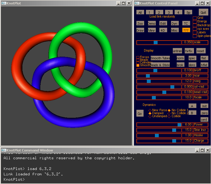
Many of the images appearing in The Knot Atlas where created using Rob Scharein's program KnotPlot. See Figure 10.
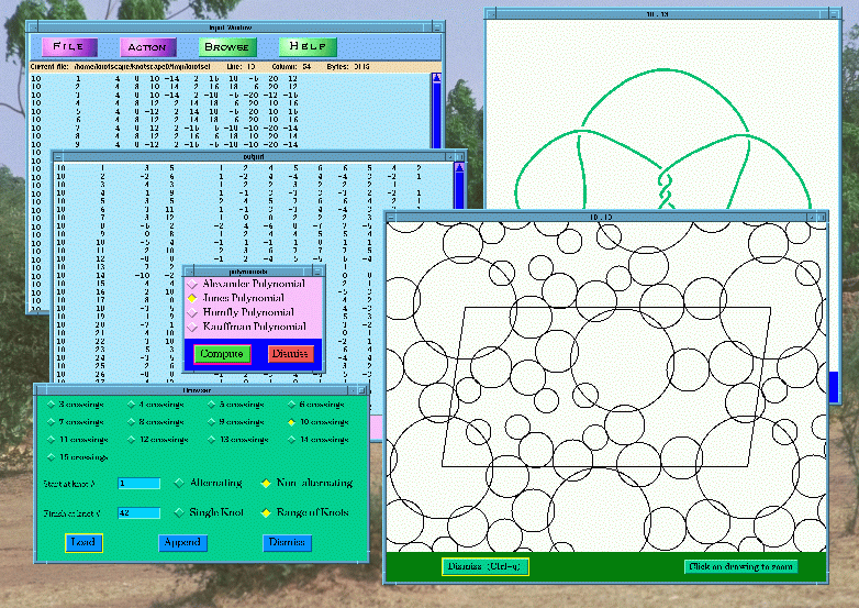
Many of the images appearing in The Knot Atlas where created using Jim Hoste's and Morwen Thistlethwaite's program Knotscape. See Figure 11.
Revision History:
About this Document ...
The html versions of this document were generated from the source files using a longish makefile that preprocesses everything using Mathematica and sed, then runs LATEX2HTML, and then postprocesses everything using perl.
![\begin{figure}\centering {
\includegraphics[width=1.5in]{figs/LinkNotation.eps}
}
\end{figure}](img18.gif)
![\begin{figure}\centering {
\includegraphics[width=2in]{figs/DTExample.eps}
}
\end{figure}](img25.gif)
![\begin{figure}\centering {
\includegraphics[height=2cm]{figs/8.18.eps}
}
\end{figure}](img38.gif)
![\begin{figure}\centering {
\includegraphics[height=2cm]{figs/5.1.eps}
\qquad\includegraphics[height=2cm]{figs/10.132.eps}
}
\end{figure}](img48.gif)
![\begin{figure}\centering {
\includegraphics[height=3cm]{figs/PDTrefoil.eps}
}
\end{figure}](img60.gif)
![\begin{figure}\centering {
\includegraphics[height=2cm]{figs/10.22.eps}
\qquad\includegraphics[height=2cm]{figs/10.35.eps}
}
\end{figure}](img89.gif)