 T(7,2) |
 T(9,2) |
| © | Dror Bar-Natan: The Knot Atlas: Torus Knots: |
|
 TubePlot |
This page is passe. Go here
instead!
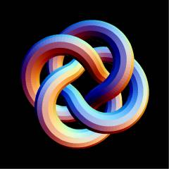
The 8-Crossing Torus Knot T(4,3)Visit T(4,3)'s page at Knotilus! |
| PD Presentation: | X5,11,6,10 X16,12,1,11 X1726 X12,8,13,7 X13,3,14,2 X8493 X9,15,10,14 X4,16,5,15 |
| Gauss Code: | {-3, 5, 6, -8, -1, 3, 4, -6, -7, 1, 2, -4, -5, 7, 8, -2} |
| Braid Representative: |
|
| Alexander Polynomial: | t-3 - t-2 + 1 - t2 + t3 |
| Conway Polynomial: | 1 + 5z2 + 5z4 + z6 |
| Other knots with the same Alexander/Conway Polynomial: | {819, ...} |
| Determinant and Signature: | {3, 6} |
| Jones Polynomial: | q3 + q5 - q8 |
| Other knots (up to mirrors) with the same Jones Polynomial: | {819, ...} |
| Coloured Jones Polynomial (in the 3-dimensional representation of sl(2); n=2): | q6 + q9 + q12 - q13 - q16 - q19 + q20 - q22 + q23 |
| A2 (sl(3)) Invariant: | q10 + q12 + 2q14 + 2q16 + 2q18 - q22 - 2q24 - 2q26 - q28 + q32 |
| Kauffman Polynomial: | - a-10 + 5a-9z - 5a-9z3 + a-9z5 - 5a-8 + 10a-8z2 - 6a-8z4 + a-8z6 + 5a-7z - 5a-7z3 + a-7z5 - 5a-6 + 10a-6z2 - 6a-6z4 + a-6z6 |
| V2 and V3, the type 2 and 3 Vassiliev invariants: | {5, 10} |
Khovanov Homology.
The coefficients of the monomials trqj
are shown, along with their alternating sums χ (fixed j,
alternation over r).
The squares with yellow highlighting
are those on the "critical diagonals", where j-2r=s+1 or
j-2r=s+1, where s=6 is the signature of
T(4,3). Nonzero entries off the critical diagonals (if
any exist) are highlighted in red.
|
0 | 1 | 2 | 3 | 4 | 5 | χ | |||||||||
| 17 | 1 | -1 | ||||||||||||||
| 15 | 1 | -1 | ||||||||||||||
| 13 | 1 | 1 | 0 | |||||||||||||
| 11 | 1 | 1 | ||||||||||||||
| 9 | 1 | 1 | ||||||||||||||
| 7 | 1 | 1 | ||||||||||||||
| 5 | 1 | 1 |
Computer Talk. The data above can be recomputed by Mathematica using the package KnotTheory`. Following setup, the sample Mathematica session below reproduces most of the above data (Mathematica system prompts in blue, human input in red, Mathematica output in black):
In[1]:= |
<< KnotTheory` |
Loading KnotTheory` (version of August 30, 2005, 10:15:35)... | |
In[2]:= | TubePlot[TorusKnot[4, 3]] |
| |
Out[2]= | -Graphics- |
In[3]:= | Crossings[TorusKnot[4, 3]] |
Out[3]= | 8 |
In[4]:= | PD[TorusKnot[4, 3]] |
Out[4]= | PD[X[5, 11, 6, 10], X[16, 12, 1, 11], X[1, 7, 2, 6], X[12, 8, 13, 7], > X[13, 3, 14, 2], X[8, 4, 9, 3], X[9, 15, 10, 14], X[4, 16, 5, 15]] |
In[5]:= | GaussCode[TorusKnot[4, 3]] |
Out[5]= | GaussCode[-3, 5, 6, -8, -1, 3, 4, -6, -7, 1, 2, -4, -5, 7, 8, -2] |
In[6]:= | BR[TorusKnot[4, 3]] |
Out[6]= | BR[3, {1, 2, 1, 2, 1, 2, 1, 2}] |
In[7]:= | alex = Alexander[TorusKnot[4, 3]][t] |
Out[7]= | -3 -2 2 3 1 + t - t - t + t |
In[8]:= | Conway[TorusKnot[4, 3]][z] |
Out[8]= | 2 4 6 1 + 5 z + 5 z + z |
In[9]:= | Select[AllKnots[], (alex === Alexander[#][t])&] |
Out[9]= | {Knot[8, 19]} |
In[10]:= | {KnotDet[TorusKnot[4, 3]], KnotSignature[TorusKnot[4, 3]]} |
Out[10]= | {3, 6} |
In[11]:= | J=Jones[TorusKnot[4, 3]][q] |
Out[11]= | 3 5 8 q + q - q |
In[12]:= | Select[AllKnots[], (J === Jones[#][q] || (J /. q-> 1/q) === Jones[#][q])&] |
Out[12]= | {Knot[8, 19]} |
In[13]:= | ColouredJones[TorusKnot[4, 3], 2][q] |
Out[13]= | 6 9 12 13 16 19 20 22 23 q + q + q - q - q - q + q - q + q |
In[14]:= | A2Invariant[TorusKnot[4, 3]][q] |
Out[14]= | 10 12 14 16 18 22 24 26 28 32 q + q + 2 q + 2 q + 2 q - q - 2 q - 2 q - q + q |
In[15]:= | Kauffman[TorusKnot[4, 3]][a, z] |
Out[15]= | 2 2 3 3 4 4 5
-10 5 5 5 z 5 z 10 z 10 z 5 z 5 z 6 z 6 z z
-a - -- - -- + --- + --- + ----- + ----- - ---- - ---- - ---- - ---- + -- +
8 6 9 7 8 6 9 7 8 6 9
a a a a a a a a a a a
5 6 6
z z z
> -- + -- + --
7 8 6
a a a |
In[16]:= | {Vassiliev[2][TorusKnot[4, 3]], Vassiliev[3][TorusKnot[4, 3]]} |
Out[16]= | {5, 10} |
In[17]:= | Kh[TorusKnot[4, 3]][q, t] |
Out[17]= | 5 7 9 2 13 3 11 4 13 4 15 5 17 5 q + q + q t + q t + q t + q t + q t + q t |
| Dror Bar-Natan: The Knot Atlas: Torus Knots: The Torus Knot T(4,3) |
|


