 10165 |
 31 |
| © | Dror Bar-Natan: The Knot Atlas: The Rolfsen Knot Table: |
|
 KnotPlot |
This page is passe. Go here
instead!
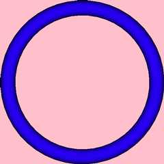
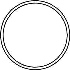
The Alternating Knot 01Also known as "The Unknot". Visit 01's page at the Knot Server (KnotPlot driven, includes 3D interactive images!) |
 KnotPlot |
| Further views: |
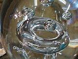 A toroidal bubble in glass |
| PD Presentation: | Loop[1] |
| Gauss Code: | {} |
| DT (Dowker-Thistlethwaite) Code: |
|
Minimum Braid Representative:
Length is 0, width is 1 Braid index is 1 |
A Morse Link Presentation:

|
| 3D Invariants: |
|
| Alexander Polynomial: | 1 |
| Conway Polynomial: | 1 |
| Other knots with the same Alexander/Conway Polynomial: | {K11n34, K11n42, ...} |
| Determinant and Signature: | {1, 0} |
| Jones Polynomial: | 1 |
| Other knots (up to mirrors) with the same Jones Polynomial: | {...} |
| A2 (sl(3)) Invariant: | q-2 + 1 + q2 |
| HOMFLY-PT Polynomial: | 1 |
| Kauffman Polynomial: | 1 |
| V2 and V3, the type 2 and 3 Vassiliev invariants: | {0, 0} |
|
Khovanov Homology:
(The squares with yellow highlighting are those on the "critical diagonals", where j-2r=s+1 or j-2r=s+1, where s=0 is the signature of 01. Nonzero entries off the critical diagonals (if any exist) are highlighted in red.) |
|
Computer Talk. The data above can be recomputed by Mathematica using the package KnotTheory`. Following setup, the sample Mathematica session below reproduces most of the above data (Mathematica system prompts in blue, human input in red, Mathematica output in black):
In[1]:= |
<< KnotTheory` |
Loading KnotTheory` (version of August 30, 2005, 10:15:35)... | |
In[2]:= | PD[Knot[0, 1]] |
Out[2]= | PD[Loop[1]] |
In[3]:= | GaussCode[Knot[0, 1]] |
Out[3]= | GaussCode[] |
In[4]:= | DTCode[Knot[0, 1]] |
Out[4]= | DTCode[] |
In[5]:= | br = BR[Knot[0, 1]] |
Out[5]= | BR[1, {}] |
In[6]:= | {First[br], Crossings[br]} |
Out[6]= | {1, 0} |
In[7]:= | BraidIndex[Knot[0, 1]] |
Out[7]= | 1 |
In[8]:= | Show[DrawMorseLink[Knot[0, 1]]] |
| |
Out[8]= | -Graphics- |
In[9]:= | #[Knot[0, 1]]& /@ {SymmetryType, UnknottingNumber, ThreeGenus, BridgeIndex, SuperBridgeIndex, NakanishiIndex} |
Out[9]= | {, 0, 0, 1, NotAvailable, NotAvailable} |
In[10]:= | alex = Alexander[Knot[0, 1]][t] |
Out[10]= | 1 |
In[11]:= | Conway[Knot[0, 1]][z] |
Out[11]= | 1 |
In[12]:= | Select[AllKnots[], (alex === Alexander[#][t])&] |
Out[12]= | {Knot[0, 1], Knot[11, NonAlternating, 34], Knot[11, NonAlternating, 42]} |
In[13]:= | {KnotDet[Knot[0, 1]], KnotSignature[Knot[0, 1]]} |
Out[13]= | {1, 0} |
In[14]:= | Jones[Knot[0, 1]][q] |
Out[14]= | 1 |
In[15]:= | Select[AllKnots[], (J === Jones[#][q] || (J /. q-> 1/q) === Jones[#][q])&] |
Out[15]= | {Knot[0, 1]} |
In[16]:= | A2Invariant[Knot[0, 1]][q] |
Out[16]= | -2 2 1 + q + q |
In[17]:= | HOMFLYPT[Knot[0, 1]][a, z] |
Out[17]= | 1 |
In[18]:= | Kauffman[Knot[0, 1]][a, z] |
Out[18]= | 1 |
In[19]:= | {Vassiliev[2][Knot[0, 1]], Vassiliev[3][Knot[0, 1]]} |
Out[19]= | {0, 0} |
In[20]:= | Kh[Knot[0, 1]][q, t] |
Out[20]= | 1 - + q q |
| Dror Bar-Natan: The Knot Atlas: The Rolfsen Knot Table: The Knot 01 |
|
