Consider wave equation in domain $\{x>0, t>0\}$, initial conditions, and a boundary condition \begin{align} &u_{tt}-c^2 u_{xx}=f(x,t) \qquad &&x>0,\label{eq-1}\\ &u|_{t=0}=g(x) && x>0,\label{eq-2}\\ &u_t|_{t=0}=h(x) && x>0,\label{eq-3} \\ &u|_{x=0}=0. \label{eq-4} \end{align} Alternatively, instead of (\ref{eq-4}) we consider \begin{align} & u_x |_{x=0}=0.\qquad&&\qquad\quad \tag*{$(4)'$}\label{eq-4-'} \end{align} Remark. It is crucial that we consider either Dirichlet or Neumann homogeneous boundary conditions.
To deal with this problem consider first IVP on the whole line: \begin{align} &U_{tt}-c^2 U_{xx}=F(x,t) \qquad &&x>0,\label{eq-5}\\ &U|_{t=0}=G(x) && x>0,\label{eq-6}\\ &U_t|_{t=0}=H(x) && x>0,\label{eq-7} \\ \end{align} and consider $V(x,t)= \varepsilon U(-x,t)$ with $\varepsilon =\pm 1$.
Proposition 1. If $U$ satisfies (\ref{eq-5})-(\ref{eq-7}) then $V$ satisfies similar problem albeit with right-hand expression $\varepsilon F(-x,t)$, and initial functions $\varepsilon G(-x)$ and $\varepsilon H(-x)$.
Proof. Plugging $V$ into equation we use the fact that $V_t(x,t)=\varepsilon U_t (-x,t)$, $V_x(x,t)=-\varepsilon U_x (-x,t)$, $V_{tt}(x,t)=\varepsilon U_{tt} (-x,t)$, $V_{tx}(x,t)=-\varepsilon U_{tx} (-x,t)$, $V_{xx}(x,t)=\varepsilon U_{xx} (-x,t)$ etc and exploit the fact that wave equation contains only even-order derivatives with respect to $x$.
Note that if $F,G,H$ are even functions with respect to $x$, and $\varepsilon=1$ then $V(x,t)$ satisfies the same IVP as $U(x,t)$. Similarly, if $F,G,H$ are odd functions with respect to $x$, and $\varepsilon=-1$ then $V(x,t)$ satisfies the same IVP as $U(x,t)$.
However we know that solution of (\ref{eq-5})-(\ref{eq-7}) is unique and therefore $U(x,t)=V(x,t)=\varepsilon U(-x,t)$.
Therefore
If $\varepsilon=-1$ and $F,G,H$ are odd functions with respect to $x$ then $U(x,t)$ is also an odd function with respect to $x$.
If $\varepsilon=1$ and $F,G,H$ are even functions with respect to $x$ then $U(x,t)$ is also an even function with respect to $x$.
However we know that a. odd function with respect to $x$ vanishes as $x=0$; b. derivative of the even function with respect to $x$ vanishes as $x=0$
and we arrive to
Therefore
Corollary 3. a. To solve (\ref{eq-1})-(\ref{eq-3}), (\ref{eq-4}) we need to take an odd continuation of $f,g,h$ to $x<0$ and solve the corresponding IVP; b. To solve (\ref{eq-1})-(\ref{eq-3}), \ref{eq-4-'} we need to take an even continuation of $f,g,h$ to $x<0$ and solve the corresponding IVP.
So far we have not used much that we have exactly wave equation (similar argments with minor modification work for heat equation as well etc). Now we apply D'Alembert formula (5.4): \begin{multline*} u(x,t)= \frac{1}{2}\bigl( G(x+ct)+G(x-ct) \bigr) + \frac{1}{2c}\int_{x-ct} ^{x+ct} H(x')\,dx' +\\ \frac{1}{2c} \int_0^t \int _{x-c(t-t')} ^{x+c(t-t')} F(x',t')\, dx' dt' \end{multline*} and we need to take $0<x<ct$, resulting for $f=0\implies F=0$ \begin{equation} u(x,t)= \frac{1}{2}\bigl( g(ct+x)- g(ct-x) \bigr) + \frac{1}{2c}\int_{ct-x} ^{ct+x} h(x')\,dx' , \label{eq-8} \end{equation} \begin{multline} u(x,t)= \frac{1}{2}\bigl( g(ct+x)+ g(ct-x) \bigr) +\\ \frac{1}{2c}\int_0 ^{ct-x} h(x')\,dx' + \frac{1}{2c}\int_0 ^{ct+x} h(x')\,dx'\qquad \tag*{(8)'}\label{eq-8-'} \end{multline} for boundary condition (\ref{eq-4}), \ref{eq-4-'} respectively.
Example. Consider wave equation with $c=1$ and let $f=0$,
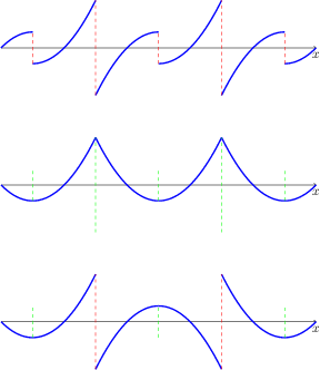
Consider the same problem albeit on interval $0<x<l$ with either Dirichlet or Neumann condition on each end. Then we need to take odd continuation through "Dirichlet end" and even continuation through "Neuman end". On figures below we have respectively Dirichlet conditions on each end (indicated by red), Neumann conditions on each end (indicated by green), and Dirichlet condition on one end (indicated by red) and Neumann conditions on another end (indicated by green). Resulting continuations are $2l$, $2l$ and $4l$ periodic respectively.
Consider multidimensional wave equation \begin{equation} u_{tt}-c^2 \Delta u=0. \label{eq-13} \end{equation} Multiplying by $u_t$ we get in the left-hand expression \begin{multline*} u_t u_{tt}-c^2 u\nabla^2 u= \partial_t \bigl(\frac{1}{2}u_t^2 \bigr)+ \nabla \cdot (-c^2 u_t \nabla u )+ c^2 \nabla u_t \cdot \nabla u =\\ \partial_t \bigl(\frac{1}{2}u_t^2 + \frac{1}{2}c^2 |\nabla u|^2\bigr)+ \nabla \cdot \bigl(-c^2 u_t \nabla u \bigr) \end{multline*} So we arrive to \begin{equation} \partial_t \bigl(\frac{1}{2}u_t^2 + \frac{1}{2}c^2 |\nabla u|^2\bigr)+ \nabla \cdot \bigl(-c^2 u_t \nabla u \bigr). \label{eq-14} \end{equation} This is energy conservation law in the differential form. \begin{equation} e= \bigl(\frac{1}{2}u_t^2 + \frac{1}{2}c^2 |\nabla u|^2\bigr) \label{eq-15} \end{equation} is a density of energy and \begin{equation} \mathbf{S}=-c^2 u_t \nabla u \label{eq-16} \end{equation} is a vector of energy flow.
Then if we fix a volume (or an area in 2D case, or just an interval in 1D case) $V$ and introduce a full energy in $V$ at moment $t$ \begin{equation} E_V(t)= \iiint _V \bigl(\frac{1}{2}u_t^2 + \frac{1}{2}c^2 |\nabla u|^2\bigr)\, dV \label{eq-17} \end{equation} then \begin{equation} E_V(t_2) - E_V(t_1) + \int_{t_1}^{t_2}dt \iint_\Sigma \mathbf{S}\cdot \mathbf{n}\, d\sigma =0 \label{eq-18} \end{equation} where $\Sigma$ is the surface bounding $V$, $d\sigma$ is an element of the surface area, and $\mathbf{n}$ is an unit exterior normal to $\Sigma$.
(optional)
Similarly, Maxwell equations in vacuum are \begin{align} &\mathbf{E}_t = c\nabla \times \mathbf{H},\label{eq-19}\\ &\mathbf{H}_t = -c\nabla \times \mathbf{E},\label{eq-20}\\ &\nabla \cdot \mathbf{E}=\nabla \cdot \mathbf{H}=0.\label{eq-21} \end{align} Multiplying (\ref{eq-19}) by $\mathbf{E}$ and (\ref{eq-20}) by $\mathbf{H}$ and adding we arrive to \begin{equation*} \partial_t \bigl(\frac{1}{2}|\mathbf{E}|^2 + \frac{1}{2}|\mathbf{H}|^2\bigr)= c\bigl(\mathbf{E}\cdot \nabla \times \mathbf{H} - \mathbf{H}\cdot \nabla \times \mathbf{E}\bigr)= c\nabla \cdot \bigl(\mathbf{E}\times \mathbf{H}\bigr) \end{equation*} where the last equality follows from vector calculus.
Then \begin{equation} \partial_t \bigl(\frac{1}{2}|\mathbf{E}|^2 + \frac{1}{2}|\mathbf{H}|^2\bigr)+ \nabla \cdot \bigl(-c\mathbf{E}\times \mathbf{H}\bigr)=0. \label{eq-22} \end{equation} In the theory of electromagnetism \begin{equation} \frac{1}{2}|\mathbf{E}|^2 + \frac{1}{2}|\mathbf{H}|^2 \label{eq-23} \end{equation} is again density of energy and \begin{equation} -c \mathbf{E}\times \mathbf{H} \label{eq-24} \end{equation} is a vector of energy flow (aka Poynting vector).