

\(\newcommand{\R}{\mathbb R }\)
\(\Leftarrow\) \(\Uparrow\) \(\Rightarrow\)
In this section we are interested in functions \(\mathbf f:U\to V\), where \(U\) and \(V\) are open subsets of \(\R^n\). Such functions, which we will call transformations, can be visualized using sketches of a subset of \(U\) and its image.
We are especially interested in functions \(\mathbf f:U\to V\) as above, such that
Such a transformation \(\mathbf f\) can be thought of as a change of coordinates. Note that \(\mathbf f\) may not be linear, but a linear change of basis is an example of this.
The Inverse Function Theorem will help us identify such functions (at least locally).
A good way to visualize a transformation \(\mathbf f\) in \(2\) dimensions is to draw pairs of pictures showing
Thus, the first picture is “before \(\mathbf f\)”, and the second picture shows “after \(\mathbf f\)”.
On the left, a grid in the \((x,y)\) plane.
On the right, its image in the \((u,v)\) plane, where red curves are images of vertical lines and blue curves are images of horizontal lines. This is the \((x,y)\) plane after applying \(\mathbf f\).
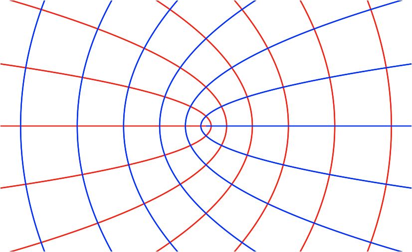
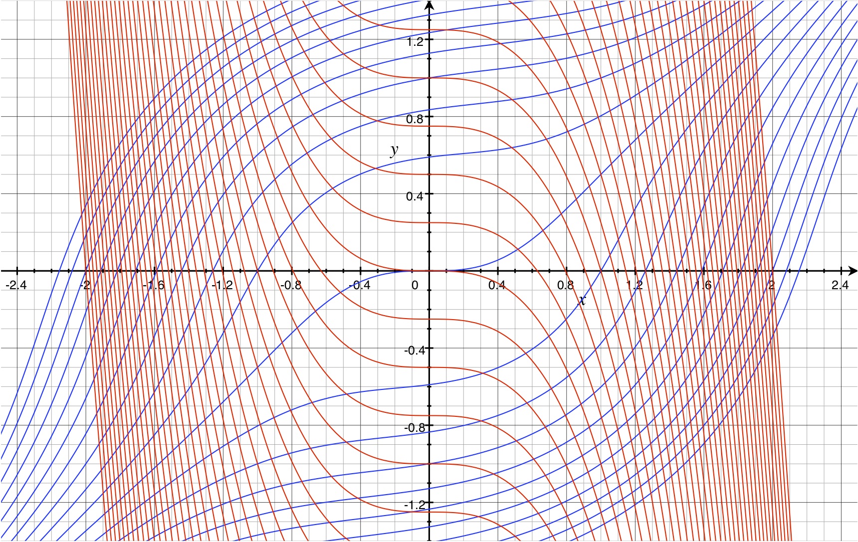
As a different way of looking at the same function, we can also picture curves in the \((x,y)\) plane (before, on the left) which correspond to a grid on in the \((u,v)\) plane (after, on the right).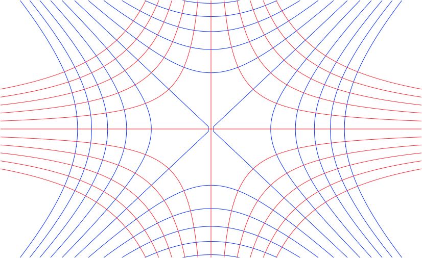

Note that the blue curves on the left are exactly level sets of \(u(x,y) = x^2-y^2\), corresponding to sets in the \(u-v\) plane where \(u\) is constant, i.e. the vertical blue lines on the right. The red curves are level sets of \(v(x,y) = 2xy\), corresponding to the horizontal red lines on the right.
An interesting feature of this function is that in both pictures, the curved lines appear to always meet at right angles.

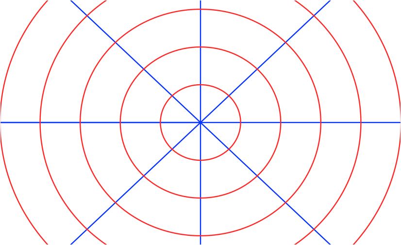
On the left, the set \(U = \{(r,\theta) : r>0, |\theta|<\pi\}\) in the \((r,\theta)\) plane. On the right, “\(\theta = \,\)constant” lines (in blue) and “\(r = \,\)constant” curves (in red) in the \((x,y)\) plane.
Spherical coordinates \((r,\theta,\varphi)\) are related to cartesian coordinates \((x,y,z)\) by \[ \begin{pmatrix} x\\y\\z \end{pmatrix}= \begin{pmatrix} r\cos\theta\sin\varphi\\\ r\sin\theta\sin\varphi\\\ r\cos\varphi \end{pmatrix} = \mathbf f(r,\theta,\varphi).\]
See the practice problems.
As above, if we want \(\mathbf f\) to be a bijection between open sets \(U\) and \(V\), it is necessary to restrict the domain and range in some appropriate way. It is common to restrict \(r>0\), \(|\theta|<\pi\), and \(0<\varphi<\pi\).
Cylindrical coordinates \((r,\theta, z)\) are related to cartesian coordinates \((x,y,z)\) by \[ \left( \begin{array}{c} x\\y\\z \end{array} \right) \ = \ \left( \begin{array}{c} r\cos\theta\\\ r\sin\theta\\\ z\end{array} \right) = \mathbf f(r,\theta,z). \] These are very closely related to polar coordinates in \(\R^2\).
The following theorem tells us when a transformation of class \(C^1\) has a local inverse of class \(C^1\).
Let \(U\) and \(V\) be open sets in \(\R^n\), and \(\mathbf f:U\to V\) a function of class \(C^1\).
Suppose that \(\mathbf a\in U\) is a point such that \[\begin{equation}\label{inv.hyp} D\mathbf f(\mathbf a) \text{ is invertible}, \end{equation}\] and let \(\mathbf b = \mathbf f(\mathbf a)\). Then there exist open sets \(M\subset U\) and \(N\subset V\) such that
Many things that we have said in Section 3.1 about the Implicit Function Theorem also apply, with some modifications, to the Inverse Function Theorem. For example:
For important and frequently-seen transformations, there are often explicit formulas for the inverse, so the Inverse Function Theorem, which guarantees the existence of an inverse without telling us what it is, may not seem very useful in these situations.
For example, this is the case for the transformation \(\mathbf f:U\to V\) that defines polar coordinates, see \(\eqref{pc}\) and \(\eqref{dr}\) above. For the \(U\) and \(V\) that we have chosen, we can write \((r,\theta) = \mathbf f^{-1}(x,y)\) — that is, we can write \(r\) and \(\theta\) as functions of \(x\) and \(y\), in a way that “inverts” \(\mathbf f:U\to V\) — as follows: \[\begin{equation}\label{rtheta} r = \sqrt{x^2+y^2}\text{ for all }(x,y)\in V, \qquad \theta = \begin{cases} {-\pi+\tan^{-1}(y/x)} &\text{ if }x<0\text{ and }y<0\\\ {-\frac\pi 2} &\text{ if }x=0\text{ and }y<0\\\ {\tan^{-1}(y/x)} &\text{ if }x>0\\\ {\frac\pi 2} &\text{ if }x=0\text{ and }y>0\\\ {\pi+\tan^{-1}(y/x)} &\text{ if }x<0\text{ and }y>0 \end{cases} \end{equation}\] (This complicated formula would be much simpler if we had chosen \(U = \{(r,\theta) : r>0, |\theta|<\pi/2\}\) and \(V = \{ (x,y) : x>0\}\). Then we can just write \(\theta = \tan^{-1}(y/x)\). This is often done, but it covers only half of the \(xy\) plane.)
The above formula can be found by elementary considerations, without using the Inverse Function Theorem. Is the Inverse Function Theorem unnecessary here?
Not entirely. The above formula is complicated, and it is hard to see, from looking at the formula, whether \(\theta\) is a differentiable function of \((x,y)\) at points where \(x=0\), and if so, what are \(\partial_x\theta\) an \(\partial_y\theta\). The easiest way to understand this is by using the Inverse Function Theorem, rather than trying to compute partial derivatives directly, starting from the complicated formula for \(\theta(x,y)\).
We can prove the theorem using the following:
To make the conclusion of Theorem 2 look more like that of the Inverse Function Theorem one can reformulate it slightly, to assert that there exist open sets \(M_0, N_0\subset \R^n\), both containing the origin, such that \(N_0\) is open, and \(\mathbf F\) is a one-to-one map from \(M_0\) onto \(N_0\).
Now, to reduce the Inverse Function Theorem to the situation considered in Theorem 2, we want to start with \(\mathbf f\) satisfying the hypotheses of the Inverse Function Theorem, and modify it to get a function \(\mathbf F\) satisfying the hypotheses of Theorem 2. To do this, let \(A = D\mathbf f(\mathbf a)\), and define \(\mathbf F:\{\mathbf x\in \R^n : \mathbf x+\mathbf a \in U\} \to \mathbb R^n\) \[\begin{equation}\label{F.def1} \mathbf F(\mathbf x) = A^{-1}\left[ \mathbf f(\mathbf x + \mathbf a) - \mathbf b\right]. \end{equation}\] One can then check that \(\mathbf F\) satisfies the hypotheses of Theorem 2, and by applying Theorem 2 to \(\mathbf F\), one can deduce that there exist sets \(M\subset U\) and \(N\subset V\) such that \(\mathbf f:M\to N\) is bijective, hence invertible.
The differentiability of \(\mathbf f^{-1}\) is more difficult to establish. The proof, which we will omit, also establishes the validity of formula \(\eqref{Dfinv}\) for \(D(\mathbf f^{-1})\). Alternately, if we already somehow know that \(\mathbf f^{-1}\) is differentiable, we can use the chain rule to check that \(\eqref{Dfinv}\) holds.
To see this, suppose that \(\mathbf f\) and \(\mathbf f^{-1}\) are both differentiable and consider the function \(\mathbf g=\mathbf f\circ \mathbf f^{-1}\). Pick any \(b\in N\subset V\) and let \(\mathbf a=\mathbf f^{-1}(\mathbf a)\). On the one hand, since \(\mathbf g(\mathbf x)=\mathbf x\) it follows that \(D\mathbf g(\mathbf b)=I\) where \(I\) is the \(n\times n\) identity matrix. On the other hand, by the chain rule, \[ D\mathbf g(\mathbf b) =D(\mathbf f\circ\mathbf f^{-1})(\mathbf b) =D\mathbf f(\mathbf f^{-1}(\mathbf b))D(\mathbf f^{-1})(\mathbf b) =D\mathbf f(\mathbf a)D(\mathbf f^{-1})(\mathbf b) \]
Thus, \(D\mathbf f(\mathbf a)D(\mathbf f^{-1})(\mathbf b)=D\mathbf g(\mathbf b)=I\). Recall from elementary linear algebra that a \(n\times n\) matrix \(A\) is invertible if and only if there exists a right inverse of \(A\), ie. a \(n\times n\) matrix \(B\) such that \(AB=I\) and in this case \(B=A^{-1}\). Hence the above equation implies that \(D(\mathbf f^{-1})(\mathbf b)=[D\mathbf f(\mathbf a)]^{-1}\) as we set out to show.
We can give a proof of the Implicit Funciton Theorem by reducing it to the Inverse Function Theorem.
Assume that \(S\) is an open subset of \(\R^{n+k}\) and that \(\mathbf F:S\to \R^k\) is a function of class \(C^1\). Assume also that \((\mathbf a, \mathbf b)\) is a point in \(S\) such that \[ \mathbf F(\mathbf a, \mathbf b) = {\bf 0} \qquad\text{ and } \qquad \det D_\mathbf y \mathbf F(\mathbf a, \mathbf b) \ne 0. \]
(i). There exist \(r_0,r_1>0\) such that for every \(\mathbf x\in \R^n\) with \(|\mathbf x-\mathbf a|< r_0\), there exists a unique \(\mathbf y\in \R^k\) with \(|\mathbf y - \mathbf b|< r_1\) such that \[\begin{equation}\label{ImFT.eq1} \mathbf F(\mathbf x, \mathbf y) = \bf0. \end{equation}\] In other words, equation \(\eqref{ImFT.eq1}\) implicitly defines a function \(\mathbf y = \mathbf f(\mathbf x)\) for \(\mathbf x\in \R^n\) near \(\mathbf a\), with \(\mathbf y = \mathbf f(\mathbf x)\) close to \(\mathbf b\). Note in particular that \(\mathbf f(\mathbf a) = \mathbf b\).
(ii). Moreover, the function \(\mathbf f:B(r_0, \mathbf a)\to B(r_1,\mathbf b)\subset \R^k\) from part (i) above is of class \(C^1\), and its derivatives may be determined by implicit differentiation.
Assume that \(\mathbf F\) satisfies the hypotheses of the Implicit Function Theorem, and define \(\mathbf G:U\to \R^{n+k}\) by \[ G(\mathbf x, \mathbf y) = (\mathbf x, \mathbf F(\mathbf x, \mathbf y)). \] Recalling that all vectors are column vectors by default, this means that \[\begin{equation}\label{G.def} G(\mathbf x, \mathbf y) = \left( \begin{array}{c} x_1\\\ \vdots\\\ x_n\\\ F_1(\mathbf x, \mathbf y)\\\ \vdots\\\ F_k(\mathbf x, \mathbf y) \end{array} \right) . \end{equation}\]
Claim 1. \(\det D\mathbf G(\mathbf a, \mathbf b) = \det D_y\mathbf F(\mathbf a, \mathbf b)\).
This is a linear algebra exercise. Note that \[ D\mathbf G \ = \ \left( \begin{array}{ccccccc} 1&0&\cdots&0&0&\cdots &0\\\ 0&1&\cdots&0&0&\cdots &0\\\ \vdots&\vdots&\ddots&0&0&\cdots &0\\\ 0&0&\cdots&1&0&\cdots &0\\\ \partial_{x_1}F_1&\partial_2 F_1&\cdots&\partial_{x_n}F_1&\partial_{y_1}F_1&\cdots &\partial_{y_k}F_1 \\\ \vdots &\vdots&\cdots&\vdots&\vdots&\cdots &\vdots\\\ \partial_{x_1}F_k&\partial_2 F_k&\cdots&\partial_{x_n}F_k&\partial_{y_1}F_k&\cdots &\partial_{y_k}F_k \\\ \end{array} \right) . \]
Here \(D\mathbf G\) denotes the \((n+k)\times (n+k)\) matrix of derivatives of all components of \(\mathbf G\) with respect to all variables \(x_1,\ldots, x_n, y_1,\ldots, y_k\). If you recall block matrices from linear algebra, you can see why Claim 1 is true. If you want to write a detailed proof, induction on \(n\) is an option.
Thus our assumption \(\det D_y\mathbf F(\mathbf a, \mathbf b)\ne 0\) implies that \(\det D\mathbf G(\mathbf a, \mathbf b) \ne 0\). Therefore according to the Inverse Function Theorem, there are open sets \(M\subset U\) and \(N\subset \R^{n+k}\) such that \((\mathbf a, \mathbf b)\in M\) and \(\mathbf G:M\to N\) is invertible, with inverse of class \(C^1\).
Next, for \(\mathbf x\) such that \((\mathbf x, {\bf 0})\in N\), define \(\mathbf f(\mathbf x)\) by \[ \mathbf G^{-1}(\mathbf x, {\bf 0}) = (\mathbf x, \mathbf f(\mathbf x)) = \left( \begin{array}{c} x_1\\\ \vdots\\\ x_n\\\ f_1(\mathbf x) \\\ \vdots\\\ f_k(\mathbf x) \end{array} \right) . \] This \(\mathbf f\) turns out to be the implicit function whose existence we are trying to prove. Its definition says that \[ \mathbf y = \mathbf f(\mathbf x) \qquad \iff\qquad (\mathbf x,\mathbf y)\in M\text{ and }G(\mathbf x, \mathbf y) = (\mathbf x , {\bf 0}). \] And of course \(\mathbf G(\mathbf x, \mathbf y) = (\mathbf x, {\bf 0 })\) is equivalent to \(\mathbf F(\mathbf x, \mathbf y) = \bf 0\).
Since \(\mathbf G^{-1}\) is \(C^1\), the same is true of \(\mathbf f\).
To complete the proof, it is still necessary to worry about a few details related to the choice of \(r_0,r_1\) in the conclusion of the theorem, but what we have said above is the main point.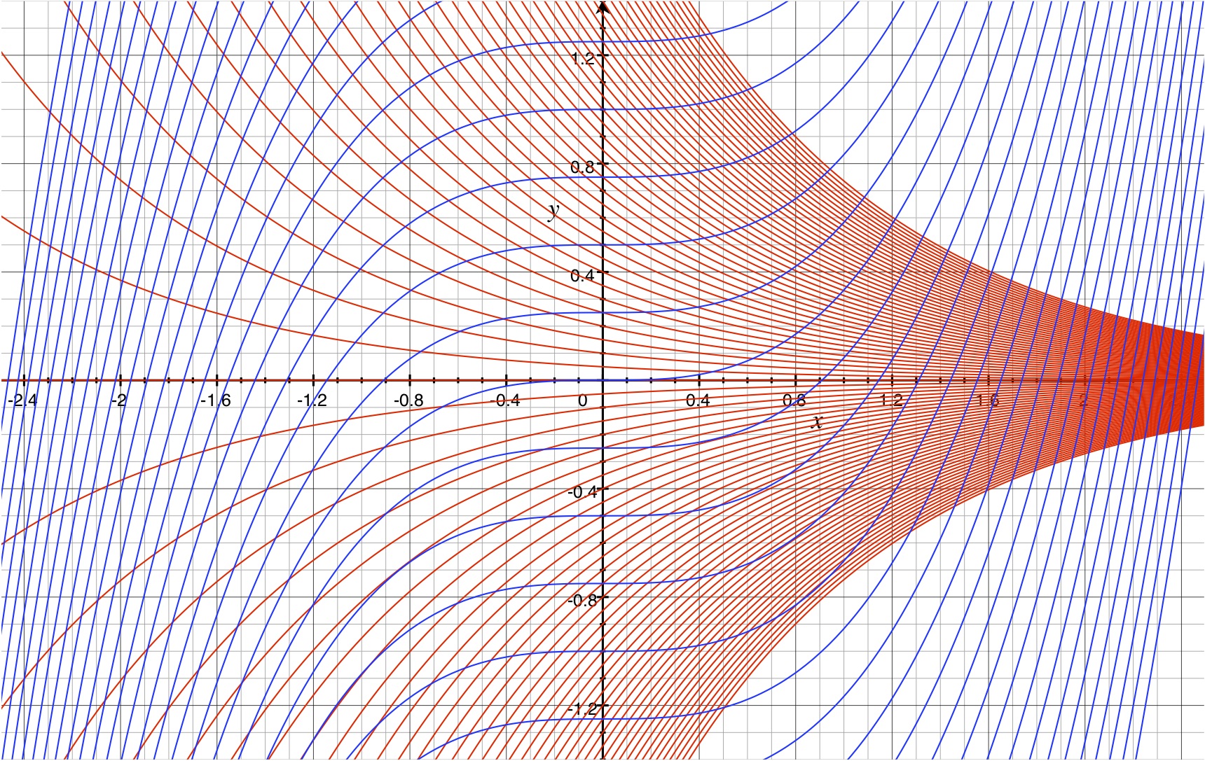
(The red curves stop where they do because filling the whole region with them would be computationally demanding, but one can imagine how they should continue.)
Same questions as in the previous problems, except that this time you should also sketch a picture showing some level curves \(u =\) constant and \(v=\) constant, for \[ (u,v) = \mathbf f(x,y) = \left(y-x^2,\frac y{1+x^2}\right), \] You might like to use different colors for level sets of \(u\) and \(v\).
For the functions \(r(x,y)\) and \(\theta(x,y)\) defined in \(\eqref{rtheta}\), check that they are both \(C^1\) functions of \((x,y)\) everywhere in their domain, and compute all partial derivatives \[ \left( \begin{array}{cc} \partial_x r & \partial_y r\\\ \partial_x \theta & \partial_y \theta \end{array}\right). \] Do this by using the Inverse Function Theorem and the easily-differentiated expressions for \((x,y)\) as functions of \((r,\theta)\). You may use that the functions defined in \(\eqref{rtheta}\) are indeed \(\mathbf f^{-1}(x,y)\), where \(\mathbf f(r,\theta)\) is defined in \(\eqref{pc}\), \(\eqref{dr}\).
Let \[ \mathbf f(x,y) = \binom{e^x(y^2-3x+1)}{x\ln(y^2+1)+y}, \] and note that \(\mathbf f(0,0) = (1,0)\)
Let \(\mathbf f:\R^3\to \R^3\) be the function that defines spherical coordinates, \[ \mathbf f(r,\theta,\varphi)\ = \ \left( \begin{array}{c} r\cos\theta\sin\varphi\\\ r\sin\theta\sin\varphi\\\ r\cos\varphi \end{array} \right) = \left( \begin{array}{c} x\\y\\z \end{array} \right) . \]
How can we restrict the domain of \(\mathbf f\) so that it is one-to one, and so that its image covers all, or almost all, of \(\R^3\)?
Describe the surfaces in \(\R^3\) that are the images of the planes \(r=\) constant, \(\theta=\) constant, \(\varphi=\) constant. (These are level sets of the inverse function \((x,y,z)\mapsto (r,\theta,\varphi) = \mathbf f^{-1}(x,y,z)\) .) If you like, you can restrict the domain of \(\mathbf f\) in a way that you have determined above.
Compute \(D\mathbf f\) and \(\det D\mathbf f\).
If we consider the domain of \(\mathbf f\) to be all of \(\R^3\), then find all points \((r,\theta, \varphi)\) at which \(\det D\mathbf f = \bf 0\). Also find the image of these points in \(xyz\) space.
Above, we have sketched a proof showing that the Implicit Function Theorem can be deduced from the Inverse Function Theorem. It is also true that the Inverse Function Theorem can be deduced from the Implicit Function Theorem. Do this; that is, assume that you know the Implicit Function Theorem is true, and use it to prove the Inverse Function Theorem.
Hint
The Inverse Function Theorem asks about the possibility of solving equations of the form \(\mathbf f(\mathbf x)= \mathbf y\) for \(\mathbf x\) as a function of \(\mathbf y\). The Implicit Function Theorem guarantees that under certain hypotheses, you can solve equations of the form \(\mathbf F(\mathbf x, \mathbf y) ={\bf 0}\) for \(\mathbf y\) as a function of \(\mathbf x\). (Note, if you want, you could swap the roles of \(\mathbf x\) and \(\mathbf y\) and solve \(\mathbf F(\mathbf y, \mathbf x) = \bf 0\) for \(\mathbf x\) as a function of \(\mathbf y\).) What this suggests is: rewrite the equation \(\mathbf f(\mathbf x) = \mathbf y\) in the form \(\mathbf F(\mathbf y, \mathbf x) = \bf0\) for a suitable function \(\mathbf F\). You may be able to use the Implicit Function Theorem to say something about solvability.
Fill in some details in the proof of the Inverse Function Theorem as sketched above. For example, verify that the function \(\mathbf F\) defined in \(\eqref{F.def1}\) satisfies the hypotheses of Theorem 2.
Fill in some details in the proof of the Implicit Function Theorem as sketched above. For example, verify that the function \(\mathbf G\) define in \(\eqref{G.def}\) satisfies
\(\det D\mathbf G(\mathbf a, \mathbf b) = \det D_y\mathbf F(\mathbf a, \mathbf b)\), as we have claimed.