
\(\newcommand{\R}{\mathbb R }\)
\(\Leftarrow\) \(\Uparrow\) \(\Rightarrow\)
There are 3 natural ways to represent a curve \(S\subseteq \R^2\):
As a graph: \[\begin{equation} \left. \begin{array}{c} S = \{ (x,y) \in \R^2: \ y = f(x) \text{ for }x\in I\}\\ \text{OR} \\ S = \{ (x,y) \in \R^2: \ x = f(y) \text{ for }y\in I\} \end{array}\right\} \label{graph} \end{equation}\] for some \(f:I\to \R\), where \(I\subseteq \R\) is an interval.
As a level set, that is, a set of the form \[\begin{equation}
S = \{ (x,y)\in U : F(x,y) = c \}
\label{locus}\end{equation}\] for some open \(U\subseteq \R^2\), some \(F:U\to \R\), and some \(c\in \R\).
This is also called the “zero locus” of \(F\) when \(c=0\).
Parametrically, that is, in the form \[\begin{equation} S = \{ \mathbf f(t) : \ t\in I \} \label{parametrically}\end{equation}\] for some interval \(I\subseteq \R\) and some \(\mathbf f:I\to \R^2\).
If \(S\) is a curve in \(\R^2\) that can be represented as the graph of a \(C^1\) function \(f:I\to \R\) for some open interval \(I\subseteq \R\), then
\(S\) can be represented as a zero locus of a function \(F\) of class \(C^1\), and
\(S\) can also be represented parametrically, as the image of a function \(\mathbf f\) of class \(C^1\).
These are true because, if \(f:I\to \R\) is a \(C^1\) function, then for example \[\begin{align}
\{ (x,y) \in \R^2: \ x\in I, y = f(x) \}
&=
\{(x,y)\in \R^2 : F(x,y)= 0\}
\nonumber \\
&=\{ \mathbf g(t): t\in I \} \nonumber
\end{align}\] for \(F(x,y) = y-f(x)\) and \(\mathbf g(t) = (t, f(t))\).
Similar considerations apply if \(S= \{ (x,y) \in \R^2: \ y\in I, x = f(y)\}\).
On the other hand, if a curve is represented as a zero locus, or parametrically, then it cannot always be represented as a graph.
For example, the Figure Eight curve below shows the set \[ S = \{(x,y)\in \R^2 : y^2 = x^2(4-x^2) \}. \] The curve can also be represented parametrically as \[ S = \{ \mathbf f(t) : t\in \R\} ,\qquad\text{ for }\mathbf f(t) = \binom{2\cos t}{2\sin 2t}. \] But cannot be represented as the graph of a \(C^1\) function. Even worse, for every \(r>0\), the set \(S\cap B(\mathbf 0; r)\), that is, the portion of the curve that is within distance \(r\) from the origin, cannot be represented as a \(C^1\) graph.
Similarly, the curve below is (a part of) \[\begin{align} S &= \{(x,y) : x^5-y^2 = 0\} \nonumber \\ &= \{ \mathbf f(t) : t\in \R\} \quad \text{ for }\ \ \mathbf f(t) = \binom{t^2}{t^5}. \nonumber \end{align}\]

This can be written as \(\{ (x,y) : x = |y|^{2/5}\}\), but the function \(f(y) = |y|^{2/5}\) is not differentiable at \(y=0\). So here too, for every \(r>0\), the set \(S\cap B(\mathbf 0; r)\) cannot be represented as a \(C^1\) graph.
Below we will say that a curve is a \(C^1\) graph as shorthand for can be represented as the graph of a \(C^1\) function.
We first consider a curve defined as a zero locus of a function \(F\).
As a result of Theorem 1, if \(\nabla F\) does not vanish at any point of \(S\), then \(S\) is not singular anywhere. By contrast, if \(\mathbf a\) is a point where \(S\) is singular, then \(\nabla F(\mathbf a) = 0\), that is, \(\mathbf a\) is a critical point.
For example, you can easily check that for both Examples 1 and 2 above, the origin is a critical point of the function that appears in the definition of the curve \(S\).
The picture below shows the set \[ S = \{(x,y)\in \R^2 : y^2 - e^{2x} + 4e^x = \alpha \}, \qquad\text{ for a particular }\alpha\in \R. \]
Determine the value of \(\alpha\).

We next consider a curve defined parametrically
The assumption that \(\mathbf f'(c)\ne \bf0\) implies that at least one component \(f_j'(c)\ne 0\), for \(j=1,2\). Let us suppose for concreteness that \(f_1'(c)\ne 0\); the other case is essentially identical.
Since \(f_1'(c)\ne 0\) and \(f_1'\) is continuous, there is some \(\varepsilon>0\) such that \(f_1'(t)\ne 0\) for \(t\in (c-\varepsilon, c+\varepsilon)\). Thus \(f_1\) is either strictly increasing or strictly decreasing in this interval, hence invertible.
Let \[ \mathbf F(t,x,y) = \left(\begin{array}{c} f_1(t) - x \\ f_2(t) - y \end{array}\right). \] Since \(f_1'(c)\ne 0\), the matrix \[ \left(\begin{array}{cc} \partial_t F_1& \partial_y F_1 \\ \partial_t F_2& \partial_y F_2 \end{array}\right) \ = \ \left(\begin{array}{cc} f_1'(t) &0 \\ f_2'(t) &-1 \end{array}\right) \] is invertible at \((t,x,y) = (c, f_1(c), f_2(c))\), so the Implicit Function Theorem implies that there exists some \(r_0, r_1>0\) and a function \(\mathbf g: (f_1(c)-r_0,f_1(c)+r_0)\to \R^2\) such that \[\begin{multline}\label{iiift} \text{ For } (t,x,y)\text{ such that }|x - f_1(c)|<r_0\text{ and } |(t,y) - (c, f_2(c))| < r_1 , \\ \mathbf F(t,x,y) = {\bf 0} \text{ if and only if }(t,y) = \mathbf g(x) \end{multline}\]
Since \(\mathbf f\) is continuous, there exists some \(r>0\) such that if \(|t-c|<r\), then \((t,x,y) = (t, f_1(t), f_2(t))\) satisfies \[ |x - f_1(c)|<r_0\text{ and } |(t,y) - (c, f_2(c))| < r_1 . \] Since \(\mathbf F(t, f_1(t), f_2(t)) = \bf0\), it follows from \(\eqref{iiift}\) that the set \[ \{ (f_1(t), f_2(t)) : |t-c|<r \} = \{ (x, g_2(x)) : x\in I\} \] where \(I\) is some subset of \((f_1(c)- r_0, f_1(c)+r_0)\).What this says is less intuitive than Theorem 1. If \(\mathbf f'(c)\ne \bf 0\), it does not say that \(S\) is regular near \(\mathbf f(c)\). It says instead only that the parametrization is regular near \(t=c\).
For example, consider again Example 1 above, where the curve can be written as \(\{\mathbf f(t) : t\in \R\}\) for \(\mathbf f(t) = \binom{2\cos t}{2\sin 2t}\). It is easy to see that
\(\mathbf f'(t)\) never vanishes. In particular, \(\mathbf f'(t)\ne \bf 0\) for \(t = \pi/2, 3\pi/2,...\).
But \(S\) looks singular near \({\bf0}\), which is \(\mathbf f(t)\) for \(t = \pi/2, 3\pi/2,...\).
This is consistent with the theorem. To see this, consider the picture below, which shows the sets \[ \{ \mathbf f(t) : |t-c|<\pi/4\} \quad\text{ for }\begin{cases} c = \pi/2 &\text{ in blue}\\ c = 3\pi/2 &\text{ in purple}. \end{cases} \]

Both the blue and the purple curves are \(C^1\) graphs. This illustrates how the parametrization can be regular even if the curve is not.
By contrast, in Example 2 above, \(\mathbf f'(t)= 0\) only for \(t=0\), and \(\mathbf f(0)\) is exactly the singular point of the curve, at the origin.
The picture below shows part of the set \[ S = \{ \mathbf f(t) : t \in \R \}, \quad\text { for } \mathbf f(t) = \binom{t^3-4t^2+5t}{t^5+6t^4+4t^3-16t^2-9t}. \] If \(\mathbf a\) denotes the point where the curve forms a cusp, then for which value of \(t\) is it true that \(\mathbf a = \mathbf f(t)\)?

As a graph: \[ \left. \begin{array}{c} S = \{ (x,y,z) \in \R^3: \ z = f(x,y) \text{ for }(x,y)\in T\}\\ \text{OR} \\ S = \{ (x,y,z) \in \R^3: \ y = f(x,z) \text{ for }(x,z)\in T\}\\ \text{OR} \\ S = \{ (x,y,z) \in \R^3: \ x = f(y,z) \text{ for }(y,z)\in T\}\\ \end{array}\right\} \] for some \(f:T\to \R\), where \(T\) is an open subset of \(\R^2\).
As a level set, that is, a set of the form \[
S \ = \ \{ (x,y,z)\in U : F(x,y,z) = c \}
\] for some open \(U\subseteq \R^3\), some \(F:U\to \R\), and some \(c\in \R\).
This is also called the “zero locus” of \(F\) when \(c=0\).
Parametrically, that is, in the form \[ S \ = \ \{ \mathbf f(\mathbf t) : \ \mathbf t\in T \} \] for some open \(T\subseteq \R^2\) and some \(\mathbf f:T\to \R^3\).
Similar to curves, if \(S\) is a surface in \(\R^3\) that can be represented as the graph of a \(C^1\) function \(f:T\to \R\) for some open interval \(T\subseteq \R^2\), then
On the other hand, if a curve is represented as a zero locus, or parametrically, then it cannot always be represented as a graph.
Below is a picture of the surface \[ S = \{ (x,y,z)\in \R^3 : y^2 + z^2 = x^2(4-x^2)\} \] It can be represented parametrically as \[ \left\{ \left( \begin{array}{c}2\cos t \\ 2\cos s \, \sin 2t \\ 2\sin s\, \sin 2t \end{array} \right) : (s,t)\in \R^2 \right\} \]

We can show that \(S\cap B(\mathbf 0;r)\) is not a \(C^1\) graph for any \(r>0\).
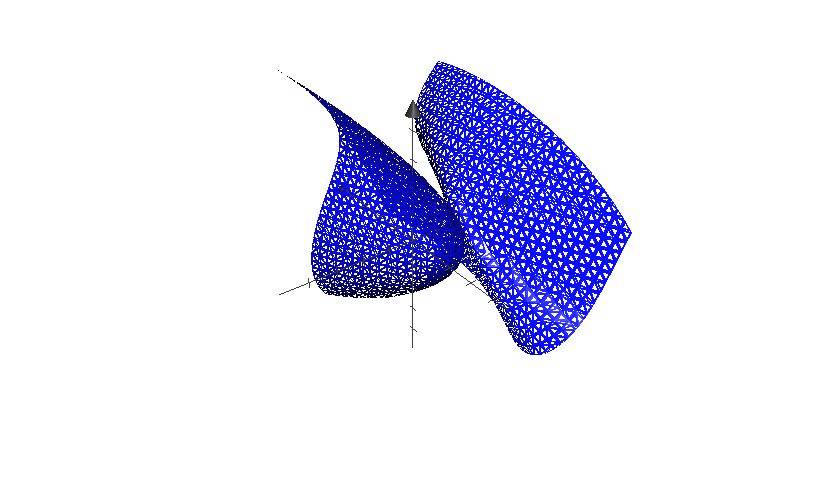
The same is true for the surface pictured below, which is \[ S = \{ (x,y,z) : x^5 - y^4-z^2=0 \} \] It can also be written parametrically as (for example) \[ \left\{ \left( f_1(s,t) , s^5 , t^5 \right) : (s,t)\in \R^2 \right\} \quad \text{ for }f_1(s,t) = \begin{cases} (s^{20}+t^{10})^{1/5}&\text{ if }(s,t)\ne (0,0)\\ 0&\text{ if }(s,t) = (0,0). \end{cases} \] It is not obvious that \(f_1\) is \(C^1\) - check that it is!

We first consider a surface defined as a zero locus of a function \(F\).
As a result of Theorem 3, if \(\mathbf a\) is a point where \(S\) is singular, then \(\nabla F(\mathbf a) = 0\), that is, \(\mathbf a\) is a critical point. And if there are no critical points of \(F\) on \(S\), then \(S\) is regular everywhere.
For example, you can easily check that for both Examples 5 above, the origin is a critical point of the function that appears in the definition of the surface \(S\).
The picture below shows the set \[
S = \{(x,y,z)\in \R^3 : x^2-4x+y^4+4y^3+6y^2+4y-z^4 = \alpha \}
\] for a particular \(\alpha\in \R\). Determine the value of \(\alpha\).

The idea of the solution is very similar to that of Example 3.
We next consider a parameterized surface.
The proof is similar in spirit to that of Theorem 2. Filling in the details is an exercise (probably a little on the hard side).
Like Theorem 2, the conclusion of the theorem is not that \(S\) is regular near \(\mathbf f(\mathbf c)\), but only that the parametrization is regular near \(\mathbf c\).Just like with curves in \(\R^2\), there are 3 common ways to represent a curve \(S\subseteq \R^3\):
As a graph: \[ \left. \begin{array}{c} S = \{ (x,y,z) \in \R^3: \ (x,y) = \mathbf f(z) \text{ for }z\in I\}\\ \text{OR} \\ S = \{ (x,y,z) \in \R^3: \ (x,z) = \mathbf f(y) \text{ for }y\in I\}\\ \text{OR} \\ S = \{ (x,y,z) \in \R^3: \ (y,z) = \mathbf f(x) \text{ for }x\in I\}\\ \end{array}\right\} \] for some \(\mathbf f:I\to \R^2\), where \(I\) is some interval.
As a level set, that is, a set of the form \[
S \ = \ \{ (x,y,z)\in U : \mathbf F(x,y,z) = \mathbf c \}
\] for some open \(U\subseteq \R^3\), some \(\mathbf F:U\to \R^2\), and some \(\mathbf c\in \R^2\).
This is also called the “zero locus” of \(\mathbf F\) when \(\mathbf c=\bf0\).
Parametrically, that is, in the form \[ S \ = \ \{ \mathbf f(t) : t\in(a,b) \} \] for some interval \((a,b)\subseteq \R\) and some \(\mathbf f:(a,b)\to \R^3\).
If \(S\) is a curve in \(\R^3\) that can be represented as the graph of a \(C^1\) function \(\mathbf f:I\to \R^2\) for some open interval \(I\subseteq \R\), then
These assertions can be proved by adapting the arguments from our discussion of curves in \(\R^2\).
On the other hand, if a curve is represented as a zero locus, or parametrically, then it cannot always be represented as a graph.
Below is a picture of the curve \[ S = \{ (x,y,z) : \mathbf F(x,y,z) = {\bf 0}\}\quad\text{ for } \mathbf F(x,y,z) = \binom{x^2-z}{y^3-z} \] It can be represented parametrically as \[ \left\{ \left( \begin{array}{c}t^3 \\t^2 \\ t^6 \end{array} \right) : t\in \R \right\} \]

It is intuitively clear that \(S\cap B(\mathbf 0;r)\) is not a \(C^1\) graph for any \(r>0\).
We use identical definitions as curves in \(\R^2\).
We first consider a curve defined as a zero locus of a function \(\mathbf F\).
As a result of Theorem 5, if \(\mathbf a\) is a point where \(S\) is singular, then \(D \mathbf F(\mathbf a)\) has rank less than \(2\).
Show that \(D\mathbf F({\bf 0})\) has rank \(1\) for Example 7.
We finally consider a parametrized curve.
The proof is similar to those of Theorems 2 and 4. Filling in the details is an exercise (probably a little on the hard side).
Like Theorems 2 and 4, the conclusion of the theorem is not that \(S\) is regular near \(\mathbf f(c)\), but only that the parametrization is regular near \(\mathbf c\).
Note that in Example 7, \(\mathbf f'(0) = \bf 0\), consistent with Theorem 6.All the above examples fall into the category of a \(m\)-dimensional “object” in \(\R^M\), where \(1\le m < M\).
For completely general \(m,M\), we can represent such an object as a level set, parametrically, or (sometimes) as a \(C^1\) graph.
Theorems 1, 3, and 5 are special cases of a general theorem. Similarly, Theorems 2, 4, and 6 are special cases of a slightly different general theorem. If you are interested, it is possible to extrapolate these general theorems from the cases considered above.
To do this by hand, you can think of the equation \(f(x,y)= c\) as a quadratic equation for \(y\), by writing it as \(4 y^2 - (8x) y + (2x^4+2-c) = 0\). This can be solved for \(y\), by using the quadratic formula. This may be time-consuming to plot by hand for several different choices of \(c\), but if you rely entirely on a computer, you will probably get some details wrong. Perhaps it is best to rely on a combination of computer and analysis.
Find all critical points of \(f\) and indicate them on your contour plot. Interpret what you see in terms of the implicit function theorem and/or theorems about curves in \(\R^2\).
If possible, determine the character of each critical point (local max, local min, or saddle point). Do the results of this exercise make sense in terms of the contour plot?
Draw a contour plot, showing the level sets \[ \{ (x,y) : F(x,y) = c\} \qquad \text{ for }c = -1, 0,1,2,3. \] If you rely entirely on a computer, you will probably get some details wrong. Also, for \(c=0\) it is easy to plot the level set, and for \(c\ne 0\) it is easy to solve for \(y\) as a function of \(x\), or vice versa, although after solving it still may be hard to plot.
Find all critical points of \(F\) and indicate them on your contour plot. Interpret what you see in terms of the implicit function theorem and/or theorems about curves in \(\R^2\).
If possible, determine the character of each critical point (local max, local min, or saddle point). Do the results of this exercise make sense in terms of the contour plot?


Find as many critical points of \(F\) as you can, and indicate them on the plot. Interpret what you see in terms of the implicit function theorem and/or theorems about curves in \(\R^2\). It may help to start by scrutinizing the graph and thinking about where the critical points should be.
For a challenge, try to find all critical points and to prove that you have done so.

On the plot, approximately determine the location of as many critical points as you can. The plot is not completely accurate, and in some places you might have to guess what it would look like if it were.
Given \(\mathbf f:(a,b) \to \R^2\), we say that \(\mathbf f\) is a regular parametrization of \(S = \{ \mathbf f(t) : a < t < b \}\) if \(\mathbf f'(t) \ne {\bf 0}\) for all \(t\in (a,b)\). For each \(\mathbf f:\R\to \R^2\) below,

Write out the proof of Theorem 3, which is a modification of the proof of Theorem 1.
Write out the proof of Theorem 4, which is a modification of the proof of Theorem 2. (It may help to consult the proof of Theorem 5.)
\(\Leftarrow\) \(\Uparrow\) \(\Rightarrow\)

This work is licensed under a Creative Commons Attribution-NonCommercial-ShareAlike 2.0 Canada License.