The Lorenz system -- An introduction to chaos

1. Introduction

In 1963, the meteorologist and mathematician E. N. Lorenz (link) discovered a remarkable system. By vastly simplifying a weather model, he discovered a 3-dimensional differential equation that exhibits "deterministic chaos".

The equation is:

\begin{aligned} \dot{x} & = \sigma(y - x) \\ \dot{y} & = rx - y - xz \\ \dot{z} & = xy - bz \end{aligned}.

He discovered that, for the parameter values \sigma = 10, b = 8/3, and r = 28, a large set of solutions are attracted to a butterfly shaped set (called the Lorenz attractor). The trajectory seems to randomly jump betwen the two wings of the butterfly. The behavior exhibited by the system is called "chaos", while this type of attractor is called a "strange attractor". For a simulation of the system, see link.

Figure 1. The Lorenz Attractor

Remark 1.1.

Roughly speaking, a system is called chaotic if its trajectory is non-periodic and exhibits sensitive dependence on initial condition.
We have seen many attracting sets such as attracting fixed points and attracting limit cycles. However, the Lorenz attractor is special because the attracting set itself is chaotic, earning the name "strange attractor".

A full mathematical analysis of the Lorenz system is very complicated. However, we can already use a lot of what we learned to understand the system. By using a simplified geometric model, we can even explain why the chaos is happening.

2. Basic analysis

2.1. Fixed points

From the fixed point equations

x = y, \quad rx - y - xz = 0, \quad xy = bz

gives us the equation

- x^3/b + rx - x = 0.

Hence x = 0 or x^2 = b(r - 1). This means the origin O = (0, 0, 0) is always a fixed point. When r > 1, we have two other fixed points C_{1, 2} = (\pm \sqrt{b(r-1)}, \pm \sqrt{b(r - 1)}, r - 1).

The differential of the vector field

D\bfF = \begin{bmatrix} - \sigma & \sigma & 0 \\ r - z & -1 & - x \\ y & x & - b \end{bmatrix}.

Let us fix \sigma and b and consider r as a parameter value. At (0, 0, 0), we have

D\bfF(O) = \begin{bmatrix} - \sigma & \sigma & 0 \\ r & -1 & 0 \\ 0 & 0 & - b \end{bmatrix}.

this shows that there is always an eigenvalue \lambda_3 = - b, while the first two eigenvalues \lambda_1, \lambda_2 are determined by the submatrix \bmat{- \sigma & \sigma \\ r & -1}. Since trace = - \sigma - 1 < 0, and \det = \sigma(1 - r), the origin undergoes a bifurcation at r = 1:

When r < 1, \lambda_1, \lambda_2 have negative real parts. Combine with \lambda_3 < 0, the origin is attracting.
When r < 1, \lambda_1, \lambda_2 have different signs. The origin is a saddle with two-dimensional attracting and one-dimensional repelling direction.

The fixed points C_{1, 2} are stable for r > 1 but not too large. At r = 1, the origin bifurcates from a stable fixed points to one unstable fixed point and two stable ones -- this is a pitchfork bifurcation.

The fixed points C_{1,2} undergoes another bifurcation at r = r_H \approx 24.74. The fixed points always have 1 negative eigenvalue and a pair of complex ones, but the real part transitions from negative real part to positive real part at r = r_H. This is an Andronov-Hopf bifurcation. A fairly complicated calculation shows that this is a subcritical bifurcation, i.e., the unstable fixed points are not surrounded by stable limit cycles.

2.2. Homoclinic bifurcation

The system undergoes another interesting bifurcation at r = r' \approx 13.926. Recall that O is a saddle with one dimensional unstable direction. The unstable manifold of O is given by two trajectories.

For r < r', the two unstable trajectories are attracted to C_1 and C_2, respectively. See Figure 2.
For r > r', the two orbits are still attracted to C_1 and C_2, but their destination has interchanged. See Figure 3.

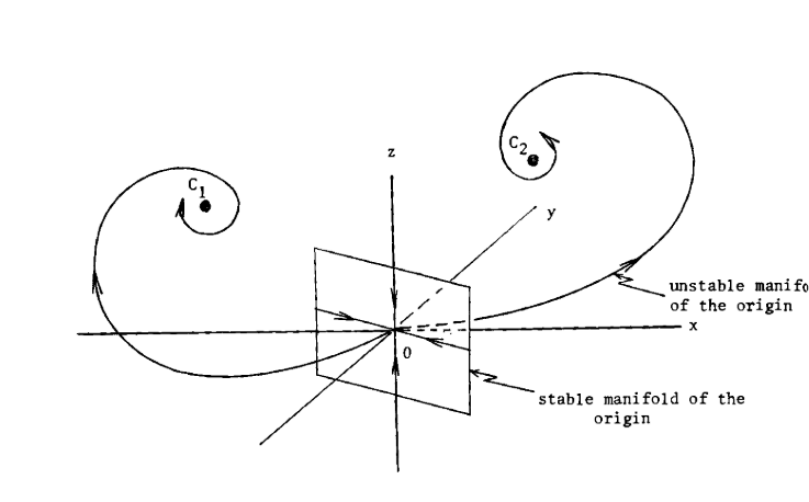
Figure 2. The unstable manifold for r < r'

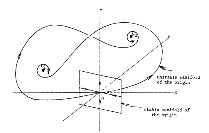
Figure 3. The unstable manifold for r > r'

The system has to go through an intermediate state of interchanging C_1 and C_2. It turns out this is a homoclinic bifurcation.

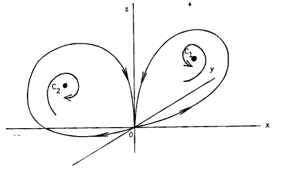
Figure 4. Homoclinic bifurcation

The crossing of unstable manifolds in Figure 3 is partially responsible for the iconic bufferfly shape.

3. The strange attractor

The picture in Figure 3 does not yet create the strange attractor, as most orbits are attracted to either C_1 and C_2. However, this changes after the Andronov-Hopf bifurcation at r = r_H \approx 24.74, as C_1, C_2 turns into unstable fixed points. As the orbits transit close to the origin, it can either move to C_1 or C_2 depending on which side of the stable manifold of the origin it's on. Since it is no longer attracted to C_1 or C_2, it goes around the fixed points and return to another transit close to the origin. It again picks one of C_1 or C_2 to trace depending on the position of crossing. These choices are highly sensitive to slight change of initial condition, as over time the orbits get separated from each other, which lead them to make different choices. This is a heuristic explanation of why chaos appears.

While all of this is happening, the orbits are being compressed together along at least one stable direction. This is why the Lorenz attractor has a two-dimension-like shape.

A geometric model of the attractor is a "branched manifold" shown below.

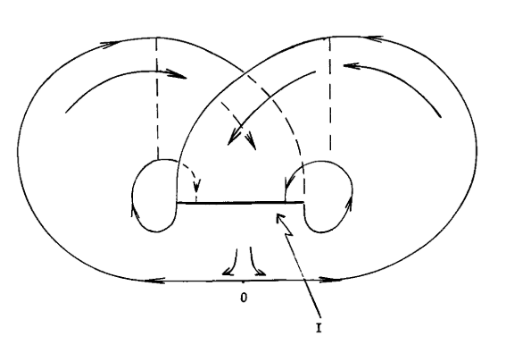
Figure 5. A geometric model of the Lorenz attractor

Pretending that the flow is defined on the branched manifold, we can study the dynamics by the Poincaré map of the section I shown in the picture. Orbits that crosses I are split into two parts depending on which side of O it's on, and when they return, the image covers part of the both halfs of I.

A graph of the Poincaré map is shown below.

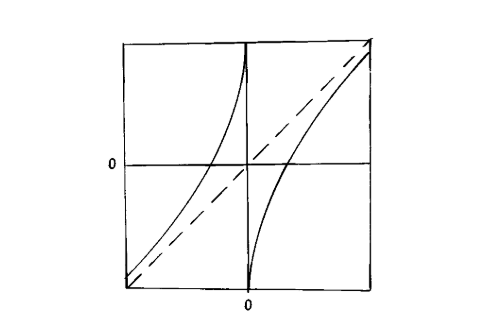
Figure 6. Poincaré map of the section I

A study of the chaotic system in the geometric Lorenz model can therefore be reduced to study the iteration of the Poincaré map in Figure 6.

4. Discrete dynamical systems

Using the example of Lorenz systems, we have seen that complex behaviour of a continuous dynamical system can be reduced to the study of iteration of a single map, called a discrete dynamical system. This will be our focus in the second half of the course.