\(\renewcommand{\R}{\mathbb R }\)
\(\Leftarrow\) \(\Uparrow\) \(\Rightarrow\)
Suppose that \(S\) is an open subset of \(\R^n\), and consider a vector-valued function \(\mathbf f:S\to \R^m\).
The idea of differentiability is essentially the same as in the case of real-valued functions: \(\mathbf f\) is differentiable at a point \(\mathbf a\in S\) if \(\mathbf f\) can be approximated by a linear map \(\R^n\to \R^m\) near \(\mathbf a\), with errors that are “smaller than linear”.
In order to write this down, we recall that it is natural to represent a linear map \(\R^n\to \R^m\) by a \(m\times n\) matrix, which acts on (column) vectors by matrix multiplication. Explicitly, a \(m\times n\) matrix \[ M = \left(\begin{array}{ccc} M_{11}& \cdots &M_{1n}\\ M_{21}& \cdots &M_{2n}\\ \vdots&\ddots&\vdots\\ M_{m1}& \cdots &M_{mn} \end{array} \right) \] represents the linear map \(\ell:\R^n\to \R^m\) defined by \[ \ell(\mathbf x)= M\mathbf x \in \R^m. \]
We also remember from linear algebra that every linear map from \(\R^n\) to \(\R^m\) can be represented by a matrix-vector multiplication like this.
Since it is natural to represent linear maps in this way, we will write the derivative at a point \(\mathbf a\in S\subseteq \R^n\) of a vector-valued function \(\mathbf f: S\to \R^m\) as a \(m\times n\) matrix.
Once we have considered this view point, the definition is very much like what we saw in the last section.
The matrix \(M\) is called the Jacobian matrix of \(\mathbf f\), named for Carl Jacobi (Prussia/Germany, 1804-1851). He is known for many advances in analysis and number theory, and gave his perspective on solving problems as “man muss immer umkehren” (“One must always invert”). We will see later that if \(M\) is a square matrix, then it is invertible if and only if \(\mathbf f\) has a differentiable inverse in a ball \(B(\mathbf f(\mathbf a); r)\). He also popularized the partial derivative notation \(\partial\).
Recall also that for a vector-valued function \(\mathbf E(\mathbf h) = (E_1(\mathbf h), \ldots, E_m(\mathbf h))\) of a variable \(\mathbf h\in \R^n\), \[ \lim_{\mathbf h\to \bf 0} \frac {{\bf E}(\mathbf h)}{|\mathbf h|} = {\bf 0} \text{ if and only if } \displaystyle\lim_{\mathbf h\to \bf 0} \dfrac {E_j(\mathbf h)}{|\mathbf h|} = 0 \text{ for all }j\in \{1,\ldots, m \}, \] as we know from Theorem 3 in Section 1.2.
The definition \(\eqref{diffnm}\) can also be written: there exists a \(m\times n\) matrix \(M\) such that \[ \lim_{\mathbf h\to {\bf 0}}\frac{\mathbf f(\mathbf a+\mathbf h) - \mathbf f(\mathbf a) - M \mathbf h}{|\mathbf h|} = {\bf 0}. \]
We will see soon that at places where \(\mathbf f\) is differentiable, there are simple expressions for the components of \(D\mathbf f(\mathbf a)\) in terms of partial derivatives of the components of \(\mathbf f\).
Recall that our default rule is every vector is a column vector unless explicitly stated otherwise, even if we write it in a way that makes it look like a row vector, such as \(\mathbf x = (x,y,z)\).
Applying this rule, if we write out all the components of \(\eqref{diffnm}\), it becomes \[\begin{equation}\label{diffnm.comp} \left( \begin{array}{c} f_1(\mathbf a+\mathbf h)\\ \vdots\\ f_m(\mathbf a+\mathbf h) \end{array} \right) = \left( \begin{array}{c} f_1(\mathbf a)\\ \vdots\\ f_m(\mathbf a) \end{array} \right) + \left(\begin{array}{ccc} M_{11}& \cdots &M_{1n}\\ \vdots&\ddots&\vdots\\ M_{m1}& \cdots &M_{mn} \end{array} \right) \left( \begin{array}{c} h_1\\ \vdots\\ h_n \end{array} \right) + \left( \begin{array}{c} E_1(\mathbf h)\\ \vdots\\ E_m(\mathbf h) \end{array} \right) , \end{equation}\] where all the components of \({\bf E}(\mathbf h)\) are smaller than linear as \(\bf h\to 0\), by which we mean that \(\lim_{\mathbf h\to \bf 0}\frac{ E_j(\mathbf h)} {|\mathbf h|} = 0\) for every \(j\).
By writing out the the \(j\)th row of \(\eqref{diffnm.comp}\), we can see that that \(\mathbf f:S\to \R^m\) is differentiable at \(\mathbf a\) if and only if, for every \(j\in \{1,\ldots, m\}\), \[\begin{equation}\label{diffnm.row} f_j(\mathbf a+\mathbf h) = f_j(\mathbf a) + \left(\begin{array}{ccc} M_{j1}& \cdots &M_{jn} \end{array} \right) \left( \begin{array}{c} h_1\\ \vdots\\ h_n \end{array} \right) + E_j(\mathbf h), \end{equation}\] where \[ \lim_{\bf h\to 0} \frac{E_j(\mathbf h)}{|\mathbf h|} = 0. \] Comparing \(\eqref{diffnm.row}\) to the definition of differentiability of a real-valued function, we see that it is equivalent to the assertion that the \(j\)th component \(f_j\) of \(\mathbf f\) is differentiable at \(\mathbf a\), for every \(j\in \{1,\ldots, m\}\). Moreover, from what we already know about differentiation of real-valued functions, we know that if \(\eqref{diffnm.row}\) holds, then it must be the case that \[ \left(\begin{array}{ccc} M_{j1}& \cdots &M_{jn} \end{array} \right) \ = \ \left(\begin{array}{ccc} \partial_1 f_j(\mathbf a)& \cdots &\partial_n f_j(\mathbf a) \end{array} \right) \] By combining this with things we already know about differentiation of scalar functions, we arrive at the following conclusions.
As in the case of real-valued functions, this theorem often provides the easiest way to check differentiability of a vector-valued function: compute all partial derivatives of all components and determine where they exist and where they are continuous. In many cases, the answer to both questions is “everywhere.”
As with real-valued functions, we say that \(\mathbf f\) is of class \(C^1\) in \(S\) (or sometimes just \(\mathbf f\) is \(C^1\)) if all partial derivatives of all components of \(\mathbf f\) exist and are continuous everywhere in \(S\).
Consider the function \(\mathbf f:\R^3\to \R^2\) defined by \[ \mathbf f(x,y,z) = \binom{f_1(x,y,z)}{f_2(x,y,z)} = \binom{ |x| +z }{ |y-1| +xz } \] Note that \(f_1\) is not differentiable when \(x=0\), and \(f_2\) is not differentiable when \(y=1\). Taking these into account, the matrix of partial derivatives at a point \((x,y,z)\) is given by \[ \left( \begin{array}{ccc}\frac x{|x|} &0&1\\ z&\frac{y-1}{|y-1|}&x \end{array} \right)\quad\text{ if }x\ne 0\text{ and }y\ne 1 \] The entries of this matrix are all continuous everywhere in \[S = \{(x,y,z)\in \R^3 : x\ne 0\text{ and }y\ne 1\},\] which is an open set, so we conclude that \(\mathbf f\) is differentiable everywhere in this set, and that the derivative \(D\mathbf f(x,y,z)\) is given by the above matrix.
We can view the case of real-valued functions as the \(m=1\) special case of \(\R^m\)-valued functions. Then, according to what we have said, for \(f:\R^n\to \R\), we should view \(Df(\mathbf a)\) as the \(1\times n\) matrix with entries \[\begin{equation}\label{Df.scalar} Df(\mathbf a) = (\partial_1 f(\mathbf a), \ldots, \partial_n f(\mathbf a)). \end{equation}\] We can recognize that this is basically the same as the gradient, although now we are insisting that \(Df\) is a row vector, which we did not do before with \(\nabla f\). The reason this occurs is that \(Df(\mathbf a)\) is not an ordinary element of \(\R^n\), but instead a (representation of a) linear map \(\R^n\to \R\). From linear algebra, we know this is a \(1\times n\) matrix or a row vector.
Another special case that arises often is the case \(n=1\), when the domain is \(1\)-dimensional. For \((a,b)\subseteq \R\), a function \(\mathbf f:(a,b)\to \R^m\) has the form \[ \mathbf f(t) = \left( \begin{array}{c} f_1(t)\\ \vdots\\ f_m(t) \end{array} \right) . \] Then if \(\mathbf f\) is differentiable at a point \(c\in (a,b)\), its derivative is a \(m\times 1\) matrix, of the form \[ \mathbf f'(c) \ = \ \ \left( \ \begin{array}{c} f_1'(c)\\ \vdots\\ f_m'(c) \end{array} \ \right) . \]
We call the image of a function \(\mathbf f:(a,b)\to \R^m\) a parametrized curve. Here are some geometric interpretations.
If \(\mathbf f\) is differentiable and \(\mathbf f'(t)\ne {\bf 0}\), then it is a vector that is tangent to the parametrized curve at \(\mathbf f(t)\).
Any (nonzero) multiple of \(\mathbf f'(t)\) is also tangent to the parametrized curve at \(\mathbf f(t)\). In particular, \(\frac{\mathbf f'(t)}{|\mathbf f'(t)|}\) is a unit tangent vector, assuming that \(\mathbf f'(t)\ne {\bf 0}\).
If we fix \(t\) and let \(h\) vary, then the straight line parametrized by \(\mathbf f(t) + h\mathbf f'(t)\) is the tangent line to the curve at \(\mathbf f(t)\).
If \(\mathbf f(t)\) represents the position of a particle at time \(t\), then \(|\mathbf f'(t)|\) is the speed of the particle at time \(t\), and \(\mathbf f'(t)\) is the velocity vector of the particle at time \(t\). The unit tangent \(\frac{\mathbf f'(t)}{|\mathbf f'(t)|}\) is the direction of motion at time \(t\).
These are illustrated by the following example.
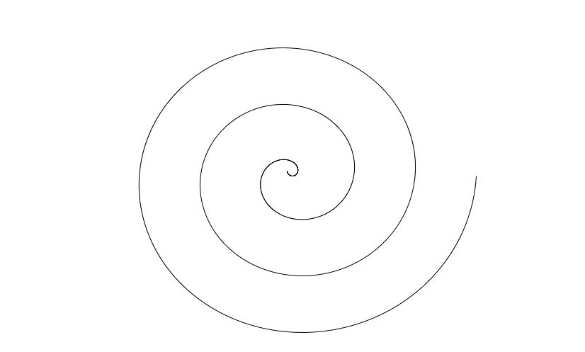
Define \(\mathbf f:\R\to \R^2\) by \(\mathbf f(t) = t\binom{\cos t}{\sin t}.\) We know that for every \(t\), \(\mathbf f(t)\) is a point whose distance from the origin is \(t\), i.e. \(|\mathbf f(t)|=t\), and that the line from the origin to \(\mathbf f(t)\) forms an angle of \(t\) radians with the positive \(x\)-axis. The image of this curve in the \(x-y\) plane is shown below, for \(t\in (-\pi/4, 6\pi)\)
The components of \(\mathbf f\) are differentiable everywhere. Thus \(\mathbf f\) is differentiable everywhere, and \[ \mathbf f'(t) = \binom{\cos t - t \sin t}{\sin t + t \cos t} . \] From the definition of the derivative, if we fix \(t\) and consider \(\mathbf f(t+h)\) as a function of \(h\), then \[ \mathbf f(t+h) \approx \mathbf f(t) + h \mathbf f'(t), \qquad\text{ for }h\text{ small,} \] in the sense that the error is smaller than linear. (That is, \({\bf E}(h)/h\to 0\) as \(h\to 0\).)
This can be seen in the picture below, which shows (in red) the sets \[\begin{equation}\label{tl} \{ \mathbf f(t) + h \mathbf f'(t), \ \ -1 < h< 1\} \end{equation}\] for several choices of \(t\), together with the same curve as above,
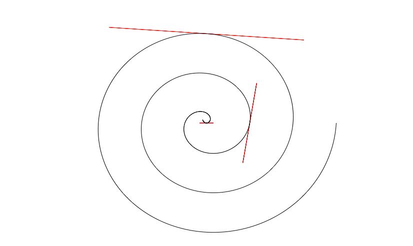
Above, in red, the set \(\eqref{tl}\) for \(t = 0, 2\pi\) and \(4\pi+\pi/2\), along with the curve defined above. From these one can see/understand the following:
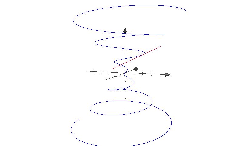
The picture below shows a portion of the curve in \(\R^3\) parametrized by \(\mathbf f(t) = (t\cos t, t\sin t, t)\), together with a segment of a tangent line \[ \{ \mathbf f(t) + h \mathbf f'(t) : -1< h < 1\} \] for a particular choice of \(t\). This is similar to Example 2.
This is also sometimes written \(d_{\mathbf a} f(\mathbf h)\). We may also neglect to mention the point \(\mathbf a\in S\) and write \(df(\mathbf h)\).
You have already used differentials when applying integration by parts: the function chosen to be \(u\) gives us the differential \(du=\frac{du}{dx}dx\), and it became helpful to think of \(du\) and \(dx\) as variables which can be manipulated algebraically.
It is common to write \[\begin{equation}\label{df.notation} df = \frac{\partial f}{\partial x_1}dx_1+\cdots +\frac{\partial f}{\partial x_n}dx_n \end{equation}\] or for example in \(2\) dimensions, \[ df = \frac{\partial f}{\partial x}dx +\frac{\partial f}{\partial y}dy. \] You can think of this as conventional notation. It was introduced by Augustin-Louis Cauchy (see problem set 2), along with the formal definition of the derivative as a limit. It is very valuable to solving differential equations and interpreting physical implications of dynamic systems. For us, the important reason to introduce this notation is that it allows us state the Chain Rule in a concise and memorable way, without a lot of messy notation.The definition of the Jacobian matrix implies that if \(\mathbf f\) is differentiable at \(\mathbf a\), then \[ \mathbf f(\mathbf a+\mathbf h) \approx \mathbf f(\mathbf a) + [D\mathbf f(\mathbf a)]\mathbf h, \qquad\text{ for $\mathbf h$ small}. \] Hence, the Jacobian matrix generalizes the idea that the derivative gives the best linear approximation to a function. This can be used to compute approximate values of functions.
Let \(f(x,y,z) = x y \sin(x^2 z)\). Estimate the numerical value of \(f(1.1,1.9,3)\).
Let \(\mathbf f(x,y)=(x\log(y),y\log(x))\). Estimate the numerical value of \(f(1.1,0.9)\).
Solution.
Write \((1.1,0.9)=\mathbf a+\mathbf h\) for \(\mathbf a=(1,1)\) and \(\mathbf h=(0.1,-0.1)\). Since \[
D\mathbf f(1,1)=\begin{pmatrix}
\log(y) & \frac{x}{y} \\
\frac{y}{x} & \log(x)
\end{pmatrix} \bigg|_{(x,y)=(1,1)}
=\begin{pmatrix} 0 & 1 \\ 1 & 0 \end{pmatrix},
\] and \(\mathbf f(1,1)=(0,0)\),
In these two examples, the linear approximation is not necessary because we have an explicit algebraic description of our function. In many applications, you may know the value at a point and how the function changes, but have no closed form. Most interesting partial differential equations fall under this category, and this idea is the basis for the finite element method using linear approximations.
Understanding and using the derivative (i.e. the Jacobian matrix) will be crucial to later concepts, like multivariable integration and change of variables. It also appears, along with its determinant, in STA 247/257 (Probability) and APM 346 (Partial Differential Equations).
Determine all points where a function \(\mathbf f\) is differentiable, and determine \(D \mathbf f\) at all such points.
Let \(\mathbf f:\R\to \R^3\) be defined by \(\mathbf f(t)=(t\cos t, \sin t, t^2)\), and consider the curve parametrized by \(\mathbf f\).
Use the Jacobian matrix to compute the approximate value of the function \(f\) at the point \(\mathbf x\). For example
Note: In \(\eqref{pr}\) above, \(\nabla \phi, \mathbf f\) and \(\mathbf g\) are all column vectors. What is the corresponding formula for the row vector \(D\phi\) (still assuming, as usual, that \(\mathbf f\) and \(\mathbf g\) are column vectors)?
The difference between these two questions is that Theorem 1 is relevant for the first one, whereas for the second, since our assumptions only give us information about differentiability at the point \(\mathbf a\), all we can use is the definition of differentiable and of the Jacobian matrix.
\(\Leftarrow\) \(\Uparrow\) \(\Rightarrow\)

This work is licensed under a Creative Commons Attribution-NonCommercial-ShareAlike 2.0 Canada License.