Graph of graphs
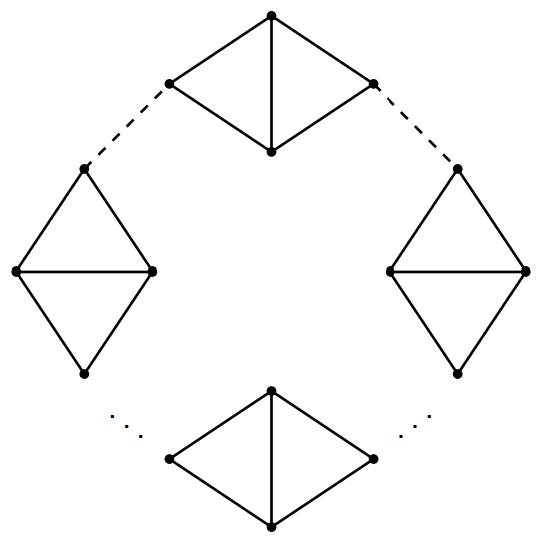
The pictures1 in this page represent the space of trivalent graphs with various number of vertices. This space has a natural geometry, namely, two graphs are close if they differ by a few local mutations.More precisely, we can give the space of graphs the structure of a graph itself. Let GG(n) be the graph whose vertices are trivalent graph with n=2k vertices and two vertices are connected by an edge if the associated graphs differ by a single Whitehead move.
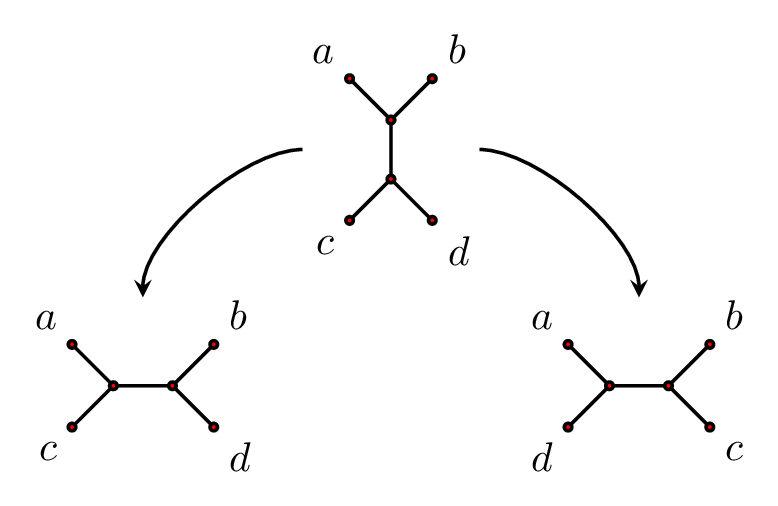 There are two Whitehead moves possible for every edge.
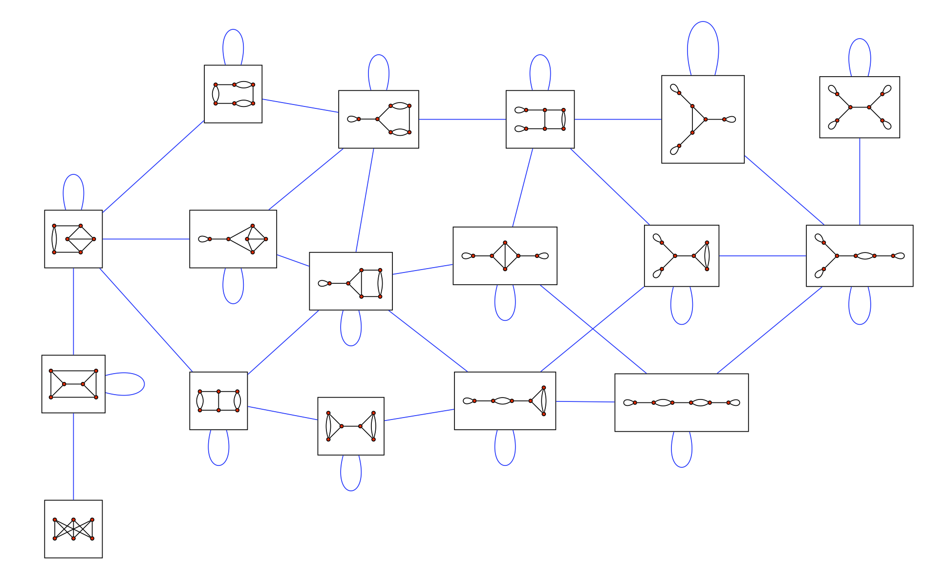 The graph GG(6).
Simple graphs
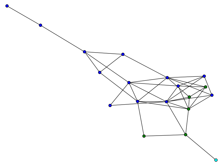
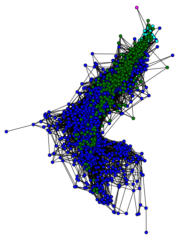
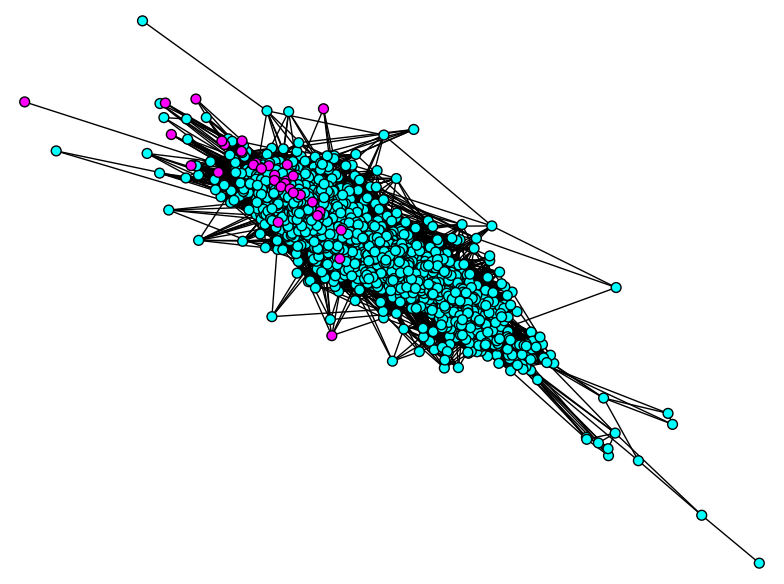
A graph is called simple if it has girth at least 3 (no loops or double edges). It was shown by Coco Zhang2 that the subgraphs GG_simple(n) and GG_not_simple(n) are both connected. Hence to simplify our discussion, we concentrate on simple graphs only. We refer to GG_simple(n) = G(n) and to the subgraph of G(n) consisting of graphs of girth at least g by G(n,g).Here are a few pictures of the graph of simple graphs. The vertices are colored by the girth of the associated graph as follows:
girth 1: black;
girth 2: white;
girth 3: blue;
girth 4: green;
girth 5: cyan; girth 6: magenta; girth 7: yellow; girth 8: red;
girth 5: cyan; girth 6: magenta; girth 7: yellow; girth 8: red;
 G(6)
G(6)
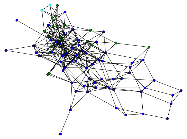
 G(8)
G(8)
 G(10)
G(10)
 G(12)
G(12)
We define G(n,k) to be the subgraph of G(n) induced by the vertices(graphs) with girth ≥ k.
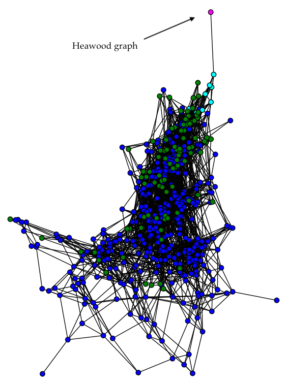 G(14)
G(14)
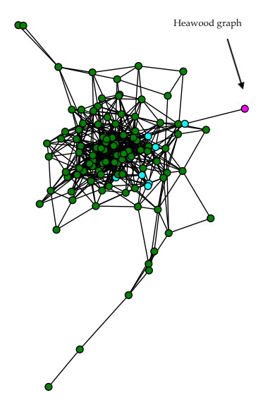 G(14,4)
 G(16)
G(16)
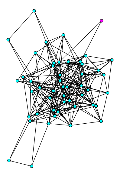 G(16,5)
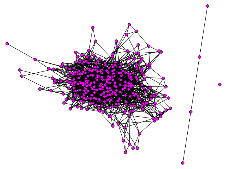
 G(18,5)
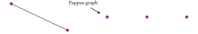 G(18,6)
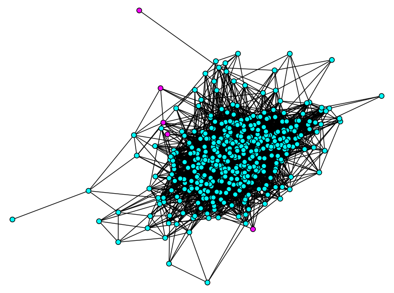
 G(20,5)
 G(20,6)
 G(22,6)
It seems like the "end" of G(n) is somewhat tree like.
c-covered graphs and connectivity of G(n,k) 3
To study the general rules of connectivity in G(n), we define the folowing term:Definition:
A graph is c-covered by short cycles (or "c-covered" for short) if every path of length c is contained in a cycle of length k, where k is the girth of graph.
Example 1:
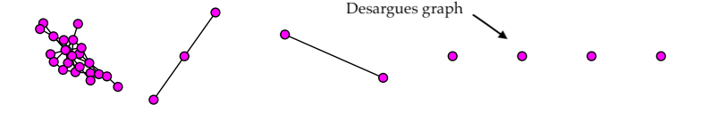
The Desargues graph (n=20, girth=6) is 3-covered by short cycles.
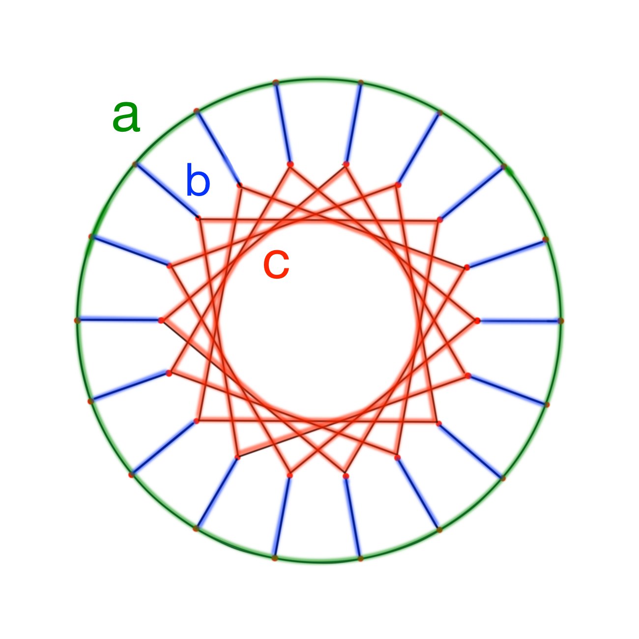
The following pictures are two representations of Desargues graphs.
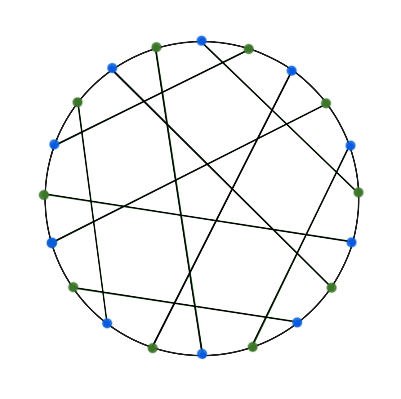 Desargues graph
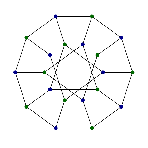 Desargues graph
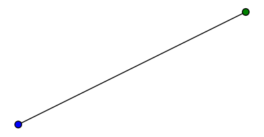
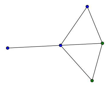
Therefore, if we pick a path P of length 3 in the Desargues graph, there exists an automorphism that maps the path to a-b-c-d depicted below. We see that there is a cycle of length 6 (a-b-c-d-e-f-a) containing the path a-b-c-d. Now, the inverse automorphism send the cycle a-b-c-d-e-f-a to a cycle that contain P. By a systole we mean a cycle that has a length equal to the girth of the graph. Thus any path of length 3 is contained in a systole and hence the Desargues graph is 3-covered.
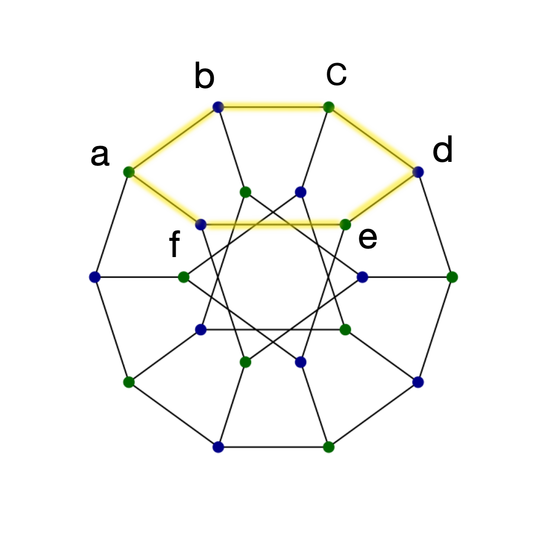 systole a-b-c-d-e-f-a
| Graph name | Number of Vertices | Girth |
| Heawood graph | 14 | 6 |
| Pappus graph | 18 | 6 |
| Desargues graph | 20 | 6 |
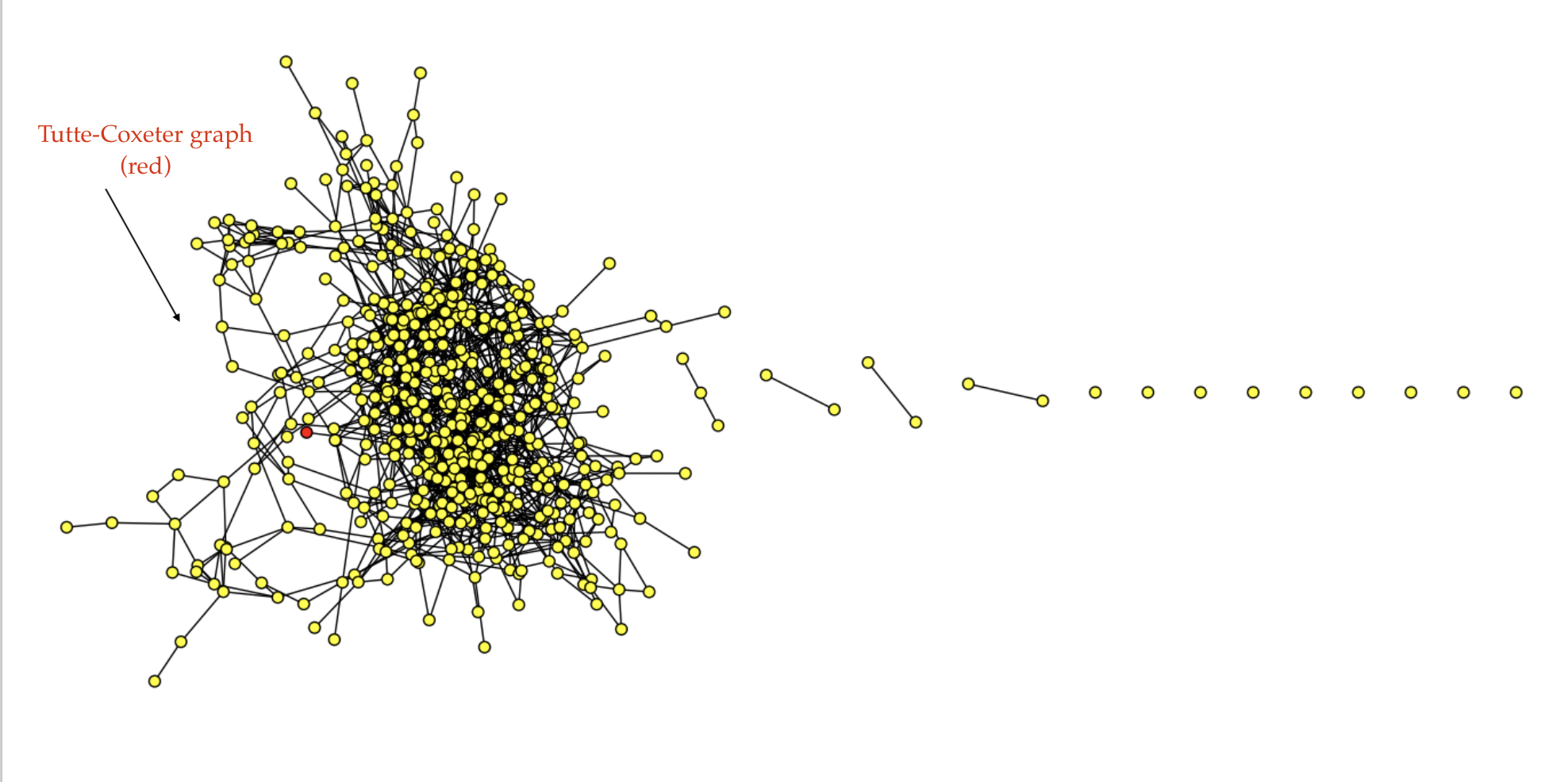
| Coxeter graph | 28 | 7 |
| Tutte-Coxeter graph | 30 | 8 |
| Foster graph | 90 | 10 |
| Biggs-Smith graph | 102 | 9 |
These special graphs are indicated in the plots of G(n) and G(n,k).
Example 2:
Generalized Petersen graph GP(3m+3, m) is 3-covered by short cycles, m ∈ N, m ≥5.
.jpg) GP(18, 5)
GP(18, 5)
Consider the case when m=5, i.e. GP(18, 5). The length of the shortest cycle is 8, thus girth = 8. And there are two types of systoles in it.
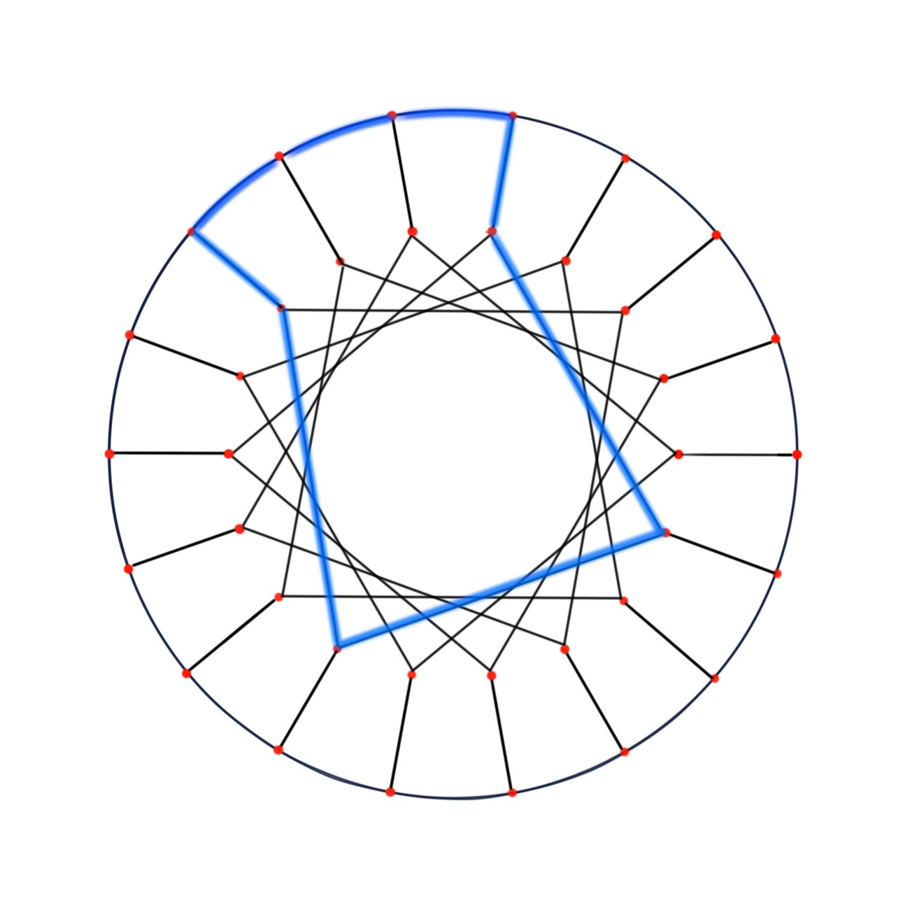 Type I
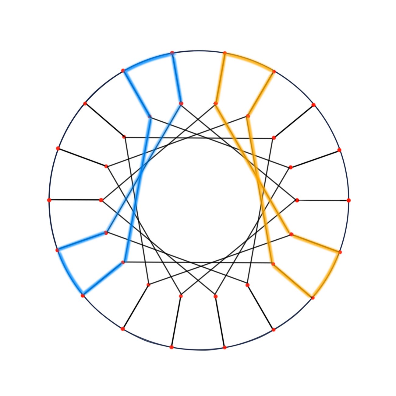 Type II
 GP(18, 5)
a-a-a, a-a-b (b-a-a), a-b-c (c-b-a), b-c-c (c-c-b), b-c-b.
a-a-a, a-a-b(b-a-a), b-c-c is contained in Type I systole;
b-c-b is contained in Type II systole;
a-b-c(c-b-a) is contained in Type I or Type II systole, depending on orientation of c.
From the argument above, any path of length 3 in GP(18, 5) is contained in a cycle of length 8. Therefore, GP(18,5) is
3-covered by short cycles. This is also true for other values of m, m ∈ N, m ≥5.
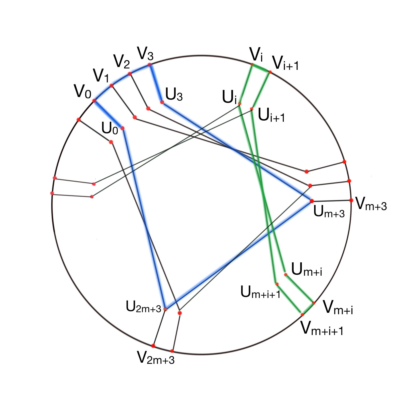 GP(3m+3, m)
Theorem:
In G(n), every 3-covered graph with girth k only connects to graphs with girth < k.
In other words, any Whithead move on 3-covered graph will decrease the girth.
Proof:
Let g be a 3-covered graph with girth k in G(n). Then every path of length 3 is contained in a cycle of length k.

Now recall that G(n,k) is a subgraph of G(n) induced by the vertices (graphs) with girth ≥ k. If G(n,k) contains only vertices (graphs) of girth k and one of these graphs is 3-covered by short cycles, then the graph is contained in a disconnected component of G(n,k).
For convenience, if the subgraph G(n,k) is disconnected and the vertices (graphs) have j different levels of girths, we call this property of G(n,k) by j-level disconnectivity. G(18,6), G(20,6) and G(22,6) above are 1-level disconnected.
Here are two examples of 2-level disconnectivity.
.png) G(24,6) contains vertices of girth 6 (cyan) and 7 (yellow)
G(24,6) contains vertices of girth 6 (cyan) and 7 (yellow)
 G(30,7) contains vertices of girth 7 (yellow) and 8 (red)
It is a question of Ci whether the property of c-covered of the vertices (graphs) in G(n,k) is related to the level of disconnectivity of G(n,k). Does a greater value of c imply more disconnectivity levels?
Here is a table of the number of trivalent graphs of a given girth. 5
| Vertices | girth = 3 | girth = 4 | girth = 5 | girth = 6 | girth = 7 | girth=8 |
| 4 | 1 | |||||
| 6 | 1 | 1 | ||||
| 8 | 3 | 2 | ||||
| 10 | 13 | 5 | 1 | |||
| 12 | 63 | 20 | 2 | |||
| 14 | 399 | 101 | 8 | 1 | ||
| 16 | 3,268 | 743 | 48 | 1 | ||
| 18 | 33,496 | 7,350 | 450 | 5 | ||
| 20 | 412,943 | 91,763 | 5,751 | 32 | ||
| 22 | 5,883,727 | 1,344,782 | 90,553 | 385 | ||
| 24 | 94,159,721 | 22,160,335 | 1,612,905 | 7,573 | 1 | |
| 26 | 1,661,723,296 | 401,278,984 | 31,297,357 | 181,224 | 3 | |
| 28 | 31,954,666,517 | 7,885,687,604 | 652,159,389 | 4,624,480 | 21 | |
| 30 | 663,988,090,257 | 166,870,266,608 | 14,499,780,660 | 122,089,998 | 545 | 1 |
| 32 | 14,814,445,040,728 | 3,781,101,495,300 | 342,646,718,608 | 3,328,899,586 | 30,368 | 0 |
| 34 | ? | ? | ? | 93,988,909,755 | 1,782,839 | 1 |
| 36 | ? | ? | ? | 2,754,127,526,293 | 95,079,080 | 3 |
Eigenvalues and bottlenecks 6
McMullen has asked whether or not the graph of graphs is an expander family. As we will see, there are multiple ways of interpreting this problem. We first define the expansion parameter of a graph \(G\) to be: \[\phi(G) := \min_{X \subset V(G)} \frac{\abs{\partial X}}{\abs{X}},\] where \(X\) is taken to be at most half the size of \(V(G)\), and \(\partial X\) denotes the boundary of \(X\). Then, we can define a family of graphs to be an expander family if \(\phi(G)\) is bounded from below.Here, we may define \(\abs{X}\) and the boundary of \(X\) in multiple ways. We may define the boundary of \(X\) to be the set of vertices adjacent to \(X\), or we may define it to be the set of edges between \(X\) and \(V(G) - X\). Also, we may define \(\abs{X}\) to be the number of vertices in \(X\), or we may define it to be the sum of the degrees in \(X\). Since the maximal degree of a vertex in GG(n) is \(O(n)\), this means that the different definitions of \(\abs{X}\) and the boundary of \(X\) may be separated by a factor of up to \(O(n)\). This leads to large differences between the corresponding definitions of the expansion parameter, so it is possible for one definition to be bounded while another definition is not. Hence, we obtain multiple different variations of McMullen's problem.
For example, if we use the "edge" definition for both \(\abs{X}\) and the boundary of \(X\), then de Peralta and Kolpakov (see below) proved that the graph of graphs is not an expander family. However, if we use the "vertex" definition instead for \(\abs{X}\), while keeping the "edge" definition for the boundary of \(X\), then McMullen's problem becomes an open problem. We will focus on this open version of the problem.
Related to this, we will informally define a bottleneck in a graph to be a partition of vertices into two sets \(X\) and \(Y\) such that the number of edges between them is small compared to \(\abs{X}\) and \(\abs{Y}\) (i.e., it produces a small expansion parameter). We will also say that a bottleneck is stronger if it leads to a smaller expansion parameter. Then, an expander family is a family of graphs without strong bottlenecks, and we want to investigate the bottlenecks of GG(n) in order to approach McMullen's problem.
In 2023, de Peralta and Kolpakov (see arXiv) made a breakthrough by discovering a bottleneck in GG(n). Their key insight is that if a cubic graph has a bridge (i.e., an edge whose removal would cause the cubic graph to become disconnected), then a Whitehead move on any edge other than the bridge would preserve the bridge because Whitehead moves are local. In other words, if we let \(X\) be the set of cubic graphs with bridges, and we let \(Y\) be the set of cubic graphs without bridges, then each vertex in \(X\) has most of its edges heading towards \(X\) again. This leads to a bottleneck between \(X\) and \(Y\).
This insight worked because a bridge is a graph structure that gets preserved by any Whitehead move away from the structure; we call any such structure a local graph structure. Then, we discovered that we can generalize this proof to other local graph structures. This is significant because it allows us to find an increasingly large number of bottlenecks in GG(n) as n increases. For example, a cycle of a certain length \(k\) is a local graph structure. Then, for all \(n \ge k\), we obtain a similar bottleneck between cubic graphs with cycles of length \(k\) and cubic graphs without cycles of length \(k\). In addition, these new bottlenecks are all independent of each other: According to background research in random graph theory, if a cubic graph \(G\) with \(n\) vertices is randomly selected, then the events "\(G\) has a 1-cycle", "\(G\) has a 2-cycle", etc. become statistically independent as \(n\) approaches infinity.
Next, it turns out that we can search for even stronger bottlenecks in GG(n) using a tool called the Laplacian matrix. The Laplacian matrix of a graph \(G\) is defined to be: \[Q(G) := D(G) - A(G),\] where \(D(G)\) is the diagonal matrix consisting of the degrees of the vertices of \(G\), and \(A(G)\) is the adjacency matrix of \(G\). Then, \(Q(G)\) has an eigenvalue of \(0\), corresponding to the constant eigenfunction. Additionally, some linear algebra shows that the remaining eigenvalues of \(Q(G)\) are strictly positive if \(G\) is connected (e.g., see Wikipedia).
To explain how the Laplacian matrix relates to bottlenecks, suppose that \(G\) has a bottleneck between two subsets of vertices \(X\) and \(Y\). If there are no edges between \(X\) and \(Y\), then we would obtain more eigenfunctions corresponding to the \(0\) eigenvalue, where each such eigenfunction is constant on \(X\) and constant on \(Y\). If \(G\) is connected and there are a few edges between \(X\) and \(Y\) instead, then it would only change these eigenvalues and eigenfunctions slightly. As a result, we would obtain a tiny positive eigenvalue, corresponding to an eigenfunction whose minimal and maximal entries indicate which "side" of the bottleneck each vertex is on. Therefore, if we search for the smallest positive eigenvalues of \(Q(G)\) and their corresponding eigenvectors, then the eigenvectors can help us find bottlenecks of \(G\).
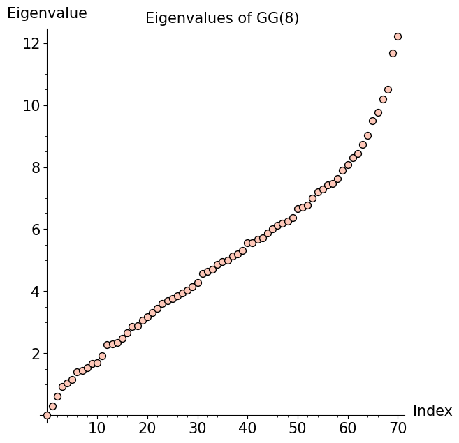
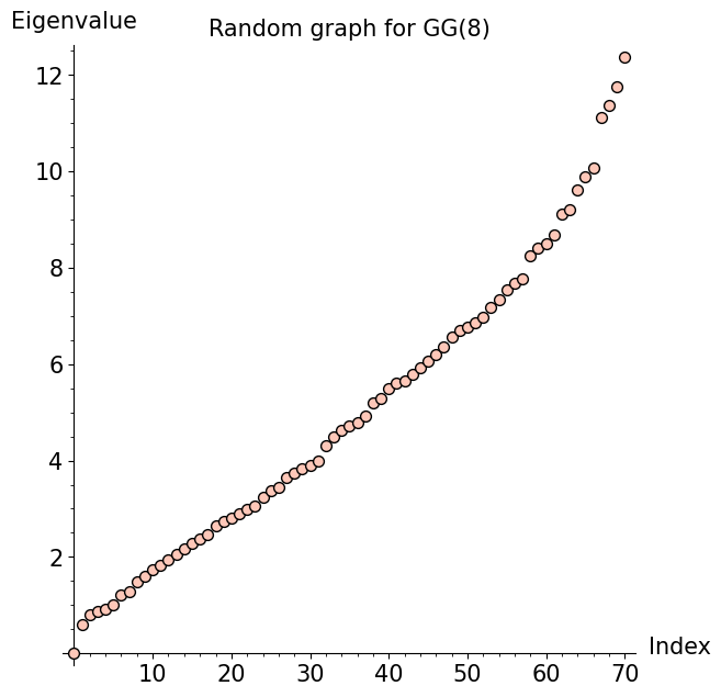
Motivated by the above discussion, we used Sage scripts to compute the first few eigenvalues and eigenvectors of GG(n) and GG_simple(n) for several values of n. We will present some interesting results from those scripts. To begin, here is a plot showing all of the eigenvalues of GG(8) (left figure), along with a plot showing the eigenvalues of a randomly generated graph (right figure) with the same number of vertices and edges as GG(8):

On the other hand, we found a different, more interesting pattern for GG(n). To illustrate, here are two plots for GG(10):
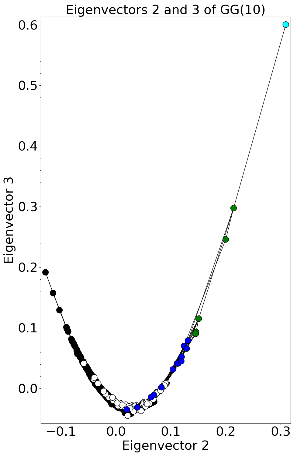
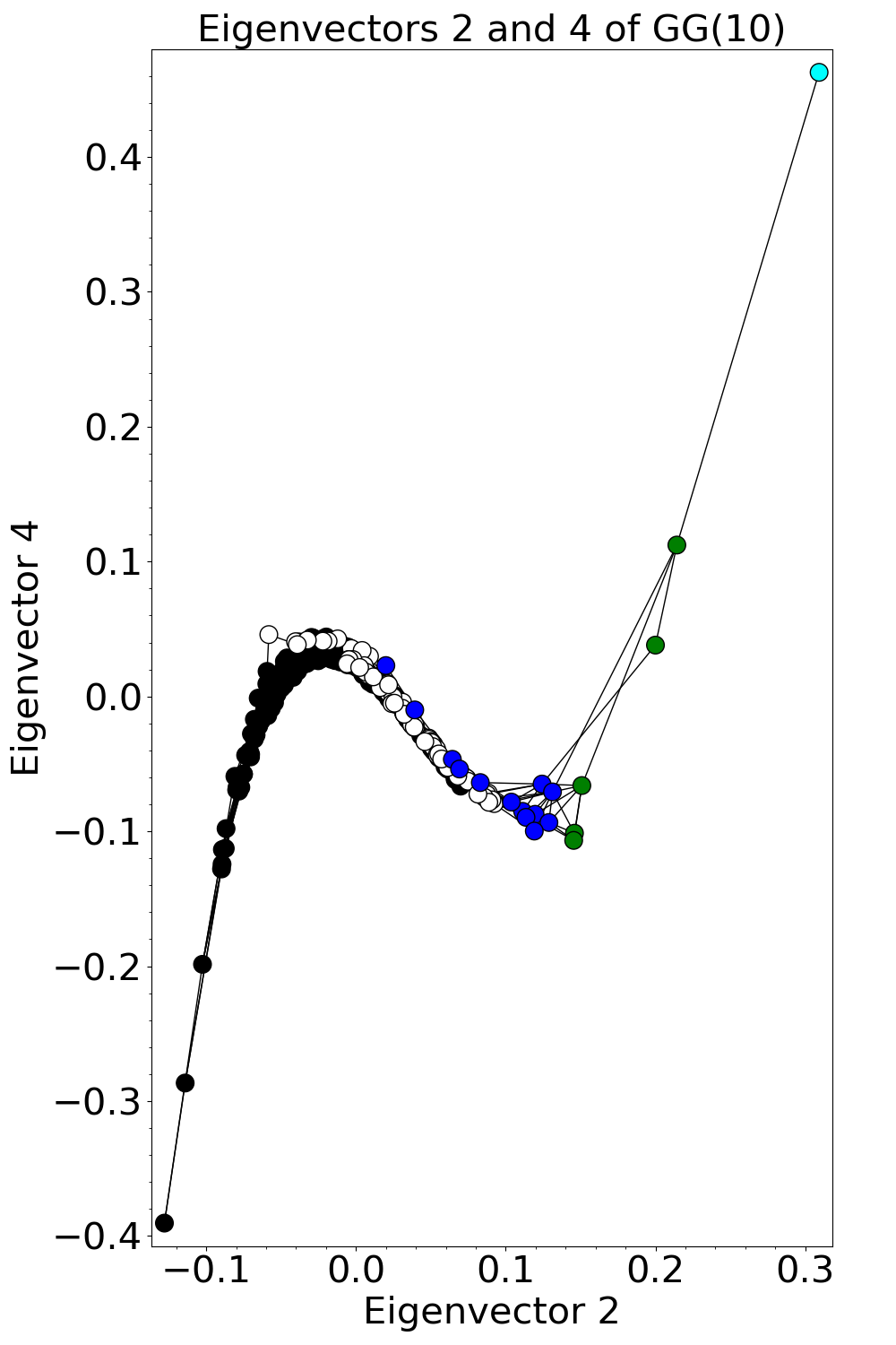
Since this result indicates that several eigenvectors of GG(n) depend on Eigenvector 2, we are highly interested in what Eigenvector 2 looks like. Based on rough statistical analyses, there may be weak correlations between the entries of Eigenvector 2 and the girth, diameter, or number of loops in a cubic graph.
Footnotes
- 1- These pictures have been produce in collaboration with Roi Docampo, Jing Tao and Ci Zhang using Sage. ↩
- 2- In 2013, Coco Zhang was a high school junior at Branksome Hall. This work was done as part of the Math Mentorship Program at the University of Toronto during the winter of 2013.↩
- 3- This section is written by Ci Zhang as part of her Work Study during the Summer and Fall 2018. ↩
- 4- Biggs, N. L.; Smith, D. H. (1971), "On trivalent graphs", Bulletin of the London Mathematical Society, 3 (2): 155–158, see here. MR 0286693. ↩
- 5- Source: http://oeis.org/A198303. See also here ↩
- 6- This section, including its images, was written by Michael Li as part of a research project funded by the NSERC-USRA in Summer 2023. ↩