Dror Bar-Natan: Odds, Ends, Unfinished:
The Manolescu-Ozsvath-Sarkar Complex
This Mathematica notebook contains and lightly documents a program I wrote in the summer of 2006. The program sets up the Manolescu-Ozsvath-Sarkar (MOS) complex and computes its homology, the "Knot Floer Homology". The comploex itself is described in detail in the article arXiv:math.GT/0607691 by Manolescu, Ozsvath and Sarkar.
The program is, as expected, a failure. The complexity of the MOS complex grows like n!, so only the Knot Floer homology of rather small knots can be computed. But thanks to the work of many other authors, the Knot Floer homology is known for all knots with up to 10 crossings and many bigger ones as well. So no new computations are available here. Yet the program is not pointless: I learned by writing it, you may learn by reading and using it, and parts of it are recyclable.
For a little while I plan to maintain, upgrade and update this notebook. Let T3 be the time now, let T2 be the time you downloaded this file and let T1 be the time defined below, in the first line of code. If (T3-T2)>(T2-T1), you should download a new copy from  (or web-search for the current location).
In[1]:=
![T1 = Date[]](HTMLFiles/index_2.gif)
Out[1]=

T0, the time stamp on the first version of this document, was {2006,8,1,20,41,33.442125}
Startup
To start, download the package KnotTheory` from The Knot Atlas site, save it on your system, change the path information as suits your system, and start executing this notebook.
In[2]:=
![AppendTo[$Path, "C:/drorbn/projects/KnotTheory/svn/trunk"] ;](HTMLFiles/index_4.gif)

Producing Planar Grid Diagrams
First some definitions:
In[4]:=
![InterlacedQ[{a_, b_}, {c_, d_}] := (Signature[{a, b}] Signature[{c, d}] Signature[{a, b, c, d}] === -1) ;](HTMLFiles/index_7.gif)
![Options[PlanarGridDiagram] = {Reduce → Infinity} ;](HTMLFiles/index_9.gif)
![PlanarGridDiagram[K_, opts___Rule] := PlanarGridDiagram[MorseLink[K], opts] ;](HTMLFiles/index_11.gif)


Let's compute the planar grid diagram of the trefoil knot:
In[9]:=
![PlanarGridDiagram[Knot[3, 1]]](HTMLFiles/index_15.gif)


Out[9]=
![PlanarGridDiagram[{5, 2}, {1, 3}, {2, 4}, {3, 5}, {4, 1}]](HTMLFiles/index_18.gif)
Each pair above describes one horizontal line in the planar grid diagram, with the first element being the position of the white dot on that line and the second element the position of the black dot.
Drawing Planar Grid Diagrams
Definitions and then examples, no need for words.
In[10]:=
![Options[Draw] = {OverlayMatrix → Null} ;](HTMLFiles/index_19.gif)
In[12]:=
![Show[Draw[PlanarGridDiagram[Knot[3, 1]]]]](HTMLFiles/index_21.gif)
![[Graphics:HTMLFiles/index_22.gif]](HTMLFiles/index_22.gif)
Out[12]=

The converter program PlanarGridDiagram applies some simplification rules to the result it gets. It is amusing to watch that happen:
In[13]:=
![MillettUnknot = PD[X[1, 10, 2, 11], X[9, 2, 10, 3], X[3, 7, 4, 6], X[15, 5, 16, 4], X[5, 17, 6, 16], X[7, 14, 8, 15], X[8, 18, 9, 17], X[11, 18, 12, 19], X[19, 12, 20, 13], X[13, 20, 14, 1]] ;](HTMLFiles/index_24.gif)
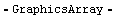
![Show[GraphicsArray[Partition[Table[Draw[PlanarGridDiagram[MillettUnknot, Reduce → k]], {k, 0, 17} ], 3]]]](HTMLFiles/index_25.gif)
![[Graphics:HTMLFiles/index_26.gif]](HTMLFiles/index_26.gif)
Out[14]=

The Minesweeper Matrix
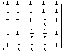
The minesweeper matrix of a planar grid diagram is the matrix of winding numbers associated with it. The brilliant terminology is due to Ken Shan.
In[15]:=
![MinesweeperMatrix[K_] := MinesweeperMatrix[PlanarGridDiagram[K]] ;](HTMLFiles/index_29.gif)
In[17]:=
![(t^MinesweeperMatrix[Knot[3, 1]]) // Reverse // MatrixForm](HTMLFiles/index_30.gif)
Out[17]//MatrixForm=
In[18]:=
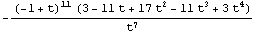
![Factor[Det[t^MinesweeperMatrix[Knot[10, 10]]]]](HTMLFiles/index_32.gif)
Out[18]=
In[19]:=
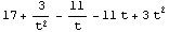
![Alexander[Knot[10, 10]][t]](HTMLFiles/index_34.gif)
Out[19]=
In[20]:=
![SetOptions[Draw, OverlayMatrix → MinesweeperMatrix] ;](HTMLFiles/index_36.gif)
![Show[GraphicsArray[{Draw[PlanarGridDiagram[Knot["K11n34"]]], Draw[PlanarGridDiagram[Knot["K11n42"]]] }]]](HTMLFiles/index_37.gif)


![[Graphics:HTMLFiles/index_40.gif]](HTMLFiles/index_40.gif)
Out[21]=
Invariance Examples for the Alexander Polynomial
In[22]:=
![MOSAlexander[K_] := Factor[Det[t^MinesweeperMatrix[K]]]](HTMLFiles/index_42.gif)
In[23]:=
![pgd = PlanarGridDiagram[K = Knot["K11n11"]]](HTMLFiles/index_43.gif)
![Draw[pgd] // Show ;](HTMLFiles/index_44.gif)
![{MOSAlexander[pgd], Alexander[K][t]}](HTMLFiles/index_45.gif)
Out[23]=
![PlanarGridDiagram[{12, 2}, {1, 10}, {3, 9}, {5, 11}, {9, 12}, {4, 8}, {2, 5}, {11, 7}, {8, 6}, {7, 4}, {10, 3}, {6, 1}]](HTMLFiles/index_46.gif)
![[Graphics:HTMLFiles/index_47.gif]](HTMLFiles/index_47.gif)
Out[25]=

Cycling
In[26]:=
![pgd1 = RotateLeft[pgd]](HTMLFiles/index_49.gif)
![Draw[pgd1] // Show ;](HTMLFiles/index_50.gif)
![MOSAlexander[pgd1]](HTMLFiles/index_51.gif)
Out[26]=
![PlanarGridDiagram[{1, 10}, {3, 9}, {5, 11}, {9, 12}, {4, 8}, {2, 5}, {11, 7}, {8, 6}, {7, 4}, {10, 3}, {6, 1}, {12, 2}]](HTMLFiles/index_52.gif)
![[Graphics:HTMLFiles/index_53.gif]](HTMLFiles/index_53.gif)
Out[28]=

Stabilization
In[29]:=
![pgd2 = pgd /. {{10, 3} → Sequence[{11, 7}, {7, 3}], j_ /; j≥7 :→ j + 1}](HTMLFiles/index_55.gif)
![Draw[pgd2] // Show ;](HTMLFiles/index_56.gif)
![MOSAlexander[pgd2]](HTMLFiles/index_57.gif)
Out[29]=
![PlanarGridDiagram[{13, 2}, {1, 11}, {3, 10}, {5, 12}, {10, 13}, {4, 9}, {2, 5}, {12, 8}, {9, 6}, {8, 4}, {11, 7}, {7, 3}, {6, 1}]](HTMLFiles/index_58.gif)
![[Graphics:HTMLFiles/index_59.gif]](HTMLFiles/index_59.gif)
Out[31]=

Commutation
In[32]:=

![Draw[pgd3] // Show ;](HTMLFiles/index_62.gif)
![MOSAlexander[pgd3]](HTMLFiles/index_63.gif)
Out[32]=
![PlanarGridDiagram[{12, 2}, {1, 10}, {3, 9}, {5, 11}, {4, 8}, {9, 12}, {2, 5}, {11, 7}, {8, 6}, {7, 4}, {10, 3}, {6, 1}]](HTMLFiles/index_64.gif)
![[Graphics:HTMLFiles/index_65.gif]](HTMLFiles/index_65.gif)
Out[34]=

The MOS complex - States and Degrees
In[35]:=
![K = TorusKnot[4, 3] ;](HTMLFiles/index_67.gif)
Note that from here on the knot K must be fixed. Every time you change it, you must re-execute all the definitions below.
In[36]:=
![Show[Draw[PlanarGridDiagram[K]]]](HTMLFiles/index_68.gif)
![[Graphics:HTMLFiles/index_69.gif]](HTMLFiles/index_69.gif)
Out[36]=

In[37]:=
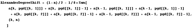
![Clear[pgd, n, MM, a, PP, WW, AlexanderDegreeShift, AlexanderDegree, x0, MaslovDegree, Boundary, AllStates, BoundaryMatrix, Rank, Betti, MOSHomology] ;](HTMLFiles/index_71.gif)
![pgd = PlanarGridDiagram[K]](HTMLFiles/index_72.gif)
Out[38]=
![PlanarGridDiagram[{1, 5}, {7, 4}, {6, 3}, {5, 2}, {4, 1}, {3, 7}, {2, 6}]](HTMLFiles/index_73.gif)
In[39]:=
![n = Length[MM = MinesweeperMatrix[pgd]]](HTMLFiles/index_74.gif)
Out[39]=

In[40]:=
![a[p1_, p2_] := a[p1, p2] = -MM[[p1 /. 0 → n, p2 /. 0 → n]] ;](HTMLFiles/index_76.gif)
Out[41]=

In[42]:=
![AlexanderDegree[x_State] := AlexanderDegree[x] = AlexanderDegreeShift + Sum[a[k, x[[k]]], {k, n} ] ;](HTMLFiles/index_79.gif)
In[43]:=
![AlexanderDegree[State[7, 6, 5, 4, 3, 2, 1]]](HTMLFiles/index_80.gif)
Out[43]=

In[44]:=
![x0 = State @@ RotateLeft[-1 + First /@ List @@ pgd] /. 0 → n](HTMLFiles/index_82.gif)
Out[44]=
![State[6, 5, 4, 3, 2, 1, 7]](HTMLFiles/index_83.gif)
In[45]:=
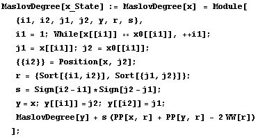
![MaslovDegree[x0] = 1 - n ;](HTMLFiles/index_84.gif)
![WW[{{i1_, i2_}, {j1_, j2_}}] := WW[{{i1, i2}, {j1, j2}}] = Length[Select[First /@ (List @@ pgd)[[Range[i1 + 1, i2]]], (j1<#≤j2) &]] ;](HTMLFiles/index_85.gif)
![PP[s_State, {{i1_, i2_}, {j1_, j2_}}] := Module[ {k, l}, Sum[l = s[[k]] ; If[i1<k<i2, 1, 1/2] * Which[j1<l<j2, 1, j1 == l || j2 == l, 1/2, True, 0], {k, i1, i2} ] ] ;](HTMLFiles/index_86.gif)
In[49]:=
![MaslovDegree[State[7, 6, 5, 4, 1, 2, 3]]](HTMLFiles/index_88.gif)
Out[49]=

In[50]:=
![AllStates[] = (State @@ #) & /@ Permutations[Range[n]] ;](HTMLFiles/index_90.gif)
![AllStates[m_, a_] := Select[AllStates[], (MaslovDegree[#] == m && AlexanderDegree[#] == a) &] ;](HTMLFiles/index_91.gif)
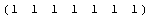
Here are all states with Maslov Degree-5 and Alexander degree 0:
In[52]:=
![AllStates[-5, 0]](HTMLFiles/index_92.gif)
Out[52]=

The MOS complex - The Differential
In[53]:=
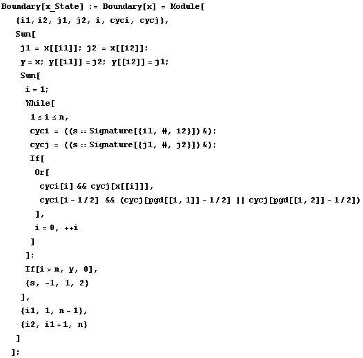
![Boundary[expr_] := expr /. x_State :→ Boundary[x] ;](HTMLFiles/index_95.gif)

In[55]:=
![bndry = Boundary[State[7, 6, 5, 4, 1, 2, 3]]](HTMLFiles/index_97.gif)
Out[55]=
![State[7, 6, 5, 4, 1, 3, 2] + State[7, 6, 5, 4, 2, 1, 3]](HTMLFiles/index_98.gif)
In[56]:=
![Boundary[bndry]](HTMLFiles/index_99.gif)
Out[56]=

In[57]:=
![BoundaryMatrix[m_, a_] := Outer[ (Boundary[#2] /. #1 → 1 /. _State → 0) &, AllStates[m - 1, a], AllStates[m, a] ] ;](HTMLFiles/index_101.gif)
In[58]:=
![BoundaryMatrix[-5, 0] // MatrixForm](HTMLFiles/index_102.gif)
Out[58]//MatrixForm=
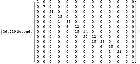
Homological computations
In[59]:=
![Rank[m_, a_] := Rank[m, a] = If[ AllStates[m, a] === {} || AllStates[m - 1, a] === {} , 0, MatrixRank[BoundaryMatrix[m, a], Modulus → 2] ] ;](HTMLFiles/index_104.gif)
![Betti[m_, a_] := Length[AllStates[m, a]] - Rank[m, a] - Rank[m + 1, a] ;](HTMLFiles/index_105.gif)
![MOSHomology[] := Outer[Betti, Union[MaslovDegree /@ AllStates[]], Union[AlexanderDegree /@ AllStates[]] ] ;](HTMLFiles/index_106.gif)
![HFK[] := Expand[Factor[Total[Flatten[Outer[ (m^#1 t^#2 Betti[#1, #2]) &, Union[MaslovDegree /@ AllStates[]], Union[AlexanderDegree /@ AllStates[]] ]]] / (1 + 1/(t m))^(n - 1) ]] ;](HTMLFiles/index_107.gif)
In[63]:=
![Rank[-5, 0]](HTMLFiles/index_108.gif)
Out[63]=

In[64]:=
![Betti[-5, 0]](HTMLFiles/index_110.gif)
Out[64]=

In[65]:=
![Timing[MOSHomology[] // MatrixForm]](HTMLFiles/index_112.gif)
Out[65]=
In[66]:=
![HFK[]](HTMLFiles/index_114.gif)
Out[66]=