$\newcommand{\erf}{\operatorname{erf}}$ $\newcommand{\const}{\mathrm{const}}$
Example 1. (Dirichlet-Dirichlet; from Lecture 12). Eigenvalue problem \begin{align} & X'' +\lambda X=0 && 0<x<l,\label{equ-13.1}\\[3pt] \label{equ-13.2}& X(0)=X(l)=0 \end{align} as eigenvalues and corresponding eigenfunctions \begin{align} & \lambda_n=\bigl(\frac{\pi n}{l}\bigr)^2,&&n=1,2,\ldots \label{equ-13.3}\\[3pt] & X_n=\sin \bigl(\frac{\pi n}{l}x\bigr). \label{equ-13.4} \end{align}
Example 2. (Neumann-Neumann). Eigenvalue problem \begin{align} & X'' +\lambda X=0 && 0<x<l,\label{equ-13.5}\\[3pt] & X'(0)=X'(l)=0\label{equ-13.6} \end{align} has eigenvalues and corresponding eigenfunctions \begin{align} & \lambda_n=\bigl(\frac{\pi n}{l}\bigr)^2,&&n=0,1,2,\ldots \label{equ-13.7}\\[3pt] & X_n=\cos \bigl(\frac{\pi n}{l}x\bigr). \label{equ-13.8} \end{align}
Example 3. (Dirichlet-Neumann) Eigenvalue problem \begin{align} & X'' +\lambda X=0 && 0<x<l,\label{equ-13.9}\\[3pt] & X(0)=X'(l)=0\label{equ-13.10} \end{align} has eigenvalues and corresponding eigenfunctions \begin{align} & \lambda_n=\bigl(\frac{\pi (2n+1)}{2l}\bigr)^2,&&n=0,1,2,\ldots \label{equ-13.11}\\[3pt] & X_n=\sin \bigl(\frac{\pi (2n+1)}{2l}x\bigr)\label{equ-13.12} \end{align} while the same problem albeit with the ends reversed (i.e. $X'(0)=X(l)=0$) has the same eigenvalues and eigenfunctions $\cos \bigl(\frac{\pi (2n+1)}{2l}x\bigr)$.
Example 4. (periodic). Eigenvalue problem \begin{align} & X'' +\lambda X=0 && 0<x<l,\label{equ-13.13}\\[3pt] & X(0)=X(l), \quad X'(0)=X'(l)\label{equ-13.14} \end{align} has eigenvalues and corresponding eigenfunctions \begin{align} & \lambda_0=0,\label{equ-13.15}\\[3pt] & X_0=1,\label{equ-13.16}\\ & \lambda_{2n}=\lambda_{2n+1}=\bigl(\frac{\pi n}{2l}\bigr)^2,&&n=1,2,\ldots \label{equ-13.17}\\[3pt] & X_{2n}=\cos \bigl(\frac{2\pi n}{l}x\bigr), && X_{2n}=\sin \bigl(\frac{2\pi n}{l}x\bigr).\label{equ-13.18} \end{align} Alternatively, as all eigenvalues but $0$ have multiplicity $2$ one can select \begin{align} & \lambda_n=\bigl(\frac{2\pi n}{l}\bigr)^2,&&n=\ldots, -2,-1,0, 1,2,\ldots \label{equ-13.19}\\[3pt] & X_{n}=\exp \bigl(\frac{2\pi n}{l}i x\bigr).\label{equ-13.20} \end{align}
Example 5. (quasiperiodic). Eigenvalue problem \begin{align} & X'' +\lambda X=0 && 0<x<l,\label{equ-13.21}\\[3pt] & X(0)=e^{-ikl}X(l), \quad X'(0)=X'(l)e^{-ikl}X(l)\label{equ-13.22} \end{align} with $0<k<\frac{2\pi}{l}$ has eigenvalues and corresponding eigenfunctions \begin{align} & \lambda_{n}=\bigl(\frac{2\pi n}{l}+k \bigr)^2,&& n=0,2,4,\ldots \label{equ-13.23}\\[3pt] & X_{n}=\exp \bigl(\bigl[\frac{2\pi n}{l}+k\bigr]i x\bigr), \label{equ-13.24}\\[3pt] & \lambda_{n}=\bigl(\frac{2\pi (n+1)}{l}-k \bigr)^2,&& n=1,3,5,\ldots \label{equ-13.25}\\[3pt] & X_{n}=\exp \bigl(\bigl[\frac{2\pi (n+1)}{l}-k\bigr]i x\bigr). \label{equ-13.26} \end{align} This is the simplest example of problems appearing in the description of free electrons in the crystals; much more complicated and realistic example would be Schrödinger equation \begin{equation*} X'' +\bigl(\lambda-V(x)\bigr)X=0 \end{equation*} or its $3D$-analog.
Example 6. (Robin boundary conditions). Consider eignevalue problem \begin{align} & X'' +\lambda X=0 && 0<x<l,\label{equ-13.27}\\[3pt] & X'(0)=\alpha X(0), \quad X'(l)=-\beta X(l)\label{equ-13.28} \end{align} with $\alpha\ge 0$, $\beta\ge 0$ ($\alpha+\beta>0$). Then \begin{multline} \lambda \int_0^l X^2\,dx=-\int_0^l X''X\,dx =\\ \int_0^l X'^2\,dx-X'(l)X(l) +X'(0)X(0)=\\ \int_0^l X'^2\,dx+\beta X(l)^2 +\alpha X(0)^2\qquad \label{equ-13.29} \end{multline} and $\lambda_n=\omega_n^2 $ where $\omega_n>0$ are roots of \begin{align} & \tan (\omega l)= \frac{(\alpha+\beta)\omega}{\omega^2-\alpha\beta}; \label{equ-13.30}\\ & X_n= \omega \cos (\omega_n x) +\alpha \sin (\omega_n x);\label{equ-13.31} \end{align} ($n=1,2,\ldots$).
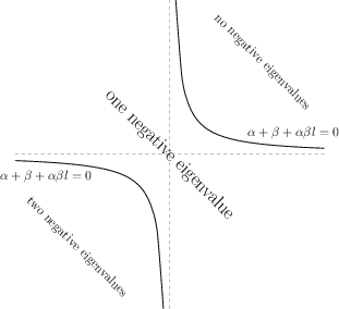
Example 7. (Robin boundary conditions (continued)). However if $\alpha $ and/or $\beta$ are negative, one or two negative eigenvalues $\lambda=-\gamma^2$ can also appear where \begin{align} & \tanh (\gamma l )= {-\frac{(\alpha + \beta)\gamma }{\gamma ^2 + \alpha\beta}}, \label{equ-13.32}\\ & X(x) = \gamma \cosh (\gamma x) + \alpha \sinh (\gamma x). \label{equ-13.33} \end{align}
To investigate when it happens, consider the threshold case of eigenvalue $\lambda=0$: then $X=cx+d$ and plugging into b.c. we have $c=\alpha d$ and $c=-\beta (d+lc)$; this system has non-trivial solution $(c,d)\ne 0$ iff $\alpha+\beta+\alpha\beta l =0$. This hyperbola divides $(\alpha,\beta)$-plane into three zones:
To calculate the number of negative eigenvalues one can either apply general variational principle Appendix B or analyze the case of $\alpha=\beta$ Appendix C.