\(\newcommand{\curl}{\operatorname{curl}}\) \(\newcommand{\div}{\operatorname{div}}\) \(\newcommand{\grad}{\operatorname{grad}}\) \(\newcommand{\R}{\mathbb R }\) \(\newcommand{\N}{\mathbb N }\) \(\newcommand{\Z}{\mathbb Z }\) \(\newcommand{\bfa}{\mathbf a}\) \(\newcommand{\bfb}{\mathbf b}\) \(\newcommand{\bfc}{\mathbf c}\) \(\newcommand{\bfe}{\mathbf e}\) \(\newcommand{\bft}{\mathbf t}\) \(\newcommand{\bff}{\mathbf f}\) \(\newcommand{\bfF}{\mathbf F}\) \(\newcommand{\bfk}{\mathbf k}\) \(\newcommand{\bfg}{\mathbf g}\) \(\newcommand{\bfn}{\mathbf n}\) \(\newcommand{\bfG}{\mathbf G}\) \(\newcommand{\bfh}{\mathbf h}\) \(\newcommand{\bfu}{\mathbf u}\) \(\newcommand{\bfv}{\mathbf v}\) \(\newcommand{\bfx}{\mathbf x}\) \(\newcommand{\bfp}{\mathbf p}\) \(\newcommand{\bfy}{\mathbf y}\) \(\newcommand{\ep}{\varepsilon}\)
\(\Leftarrow\) \(\Uparrow\) \(\Rightarrow\)
If \(S\) is a \(2\)-dimensional surface in \(\R^3\), and if \(\bfF\) is a \(C^1\) vector field, then Stokes’ Theorem relates the integral over \(S\) of \(\curl \bfF\) with the integral of \(\bfF\) over \(\partial S\), the boundary of \(S\).
For Stokes’ Theorem, we will always consider a surface \(S\) that is a subset of a smooth (or piecewise smooth) surface \(S_0\) and “the boundary of \(S\)” will be understood to mean “the boundary of \(S\) within \(S_0\).” We will occasionally call this the Stokes boundary of \(S\) to distinguish it from the definition of boundary in Section 1.1, which is different. When it is clear from the context that we are talking about the Stokes boundary, we will omit the word “Stokes”.
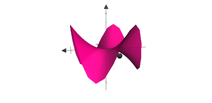
Consider \[ S = \left\{ \bfG(\bfu) : \ \bfu \in \R^2, |\bfu |\le 1\right\},\quad\text{ for } \bfG(\bfu) = (u, v, u^3-3uv^2), \] shown below:
 \(\qquad\qquad\)
A point \(\bfx\) belongs to the Stokes boundary - that is, the boundary of \(S\) within \(S_0\) - if \[ \forall r>0, \qquad B(r, \bfx)\cap S \ \ \text{ and } \ \ B(r, \bfx)\cap (S_0\setminus S)\text{ are both nonempty}. \] Thus the Stokes boundary of \(S\) is the yellow curve at the edge of \(S\), shown below.

Here it is again, with \(S_0\) omitted from the picture for clarity.

We have discussed this issue at some length, but in practice identifying the Stokes boundary of a surface \(S\) is usually very straightforward. The long discussion is to explain the difference between the Stokes boundary and our definition of boundary from Section 1.1.
For Stokes’ Theorem, we will always Suppose that \(S\) (as well as the larger smooth surface \(S_0\) that we have Supposed contains \(S\)) is oriented by a choice of the unit normal \(\bfn\). Informally, the orientation for \(\partial S\) may be described by saying that if someone walks around \(\partial S\) with their head pointing in the direction of the unit normal \(\bfn\), and with \(S\) on the left, then the Stokes orientation corresponds to the direction in which they travel around \(\partial S\).
Slightly more mathematically, this means that at a point \(\bfx\in \partial S\), if \(\bfn\) denotes the positively oriented normal to \(S_0\) and if \(\bft\) denoted the tangent to \(\partial S\) at \(\bfx\) with the Stokes orientation, then \[ \bfn\times\bft\text{ points into }S. \]
In Example 1 above, one can see that if \(S\) is oriented with \(\bfn\) pointed upwards, then the Stokes orientation for \(\partial S\) is counterclockwise (as seen from above.)
This is more generally true: \(S\) is a graph, that is, a surface parametrized by \[\begin{equation}\label{graph}
\bfG(u,v)\ \text{ of the form }\ (u, v, \phi(u,v)) , \ \
\qquad (u,v)\in R \subset \R^2,
\end{equation}\] where \(R\) is a convex subset of \(\R^2\) and also (as usual) a regular region with piecewise \(C^1\) boundary. If \(S\) is oriented with \(\bfn\) pointing upwards, then again the Stokes orientation for \(\partial S\) points in the counterclockwise direction (as seen from above) around \(\partial S\).
Many concrete problems that you will see concern surfaces \(S\) that can be put in the form , so it is a good idea to remember this basic fact about the orientation of \(\partial S\).
A formula for the orientation (optional!)
In practice, you will probably never need to write down a formula that describes the Stokes orientation of some boundary \(\partial S\). But in case you are reassured to know that such a formula exists, here it is (in the case when the surface \(S\) has a nice parametrization):
Suppose that \(R\) is regular region in \(\R^2\) contained in an open set \(R_0\), and that \(\bfG:R_0\to \R^3\) parametrizes the smooth surface \(S_0\), with its restriction to \(R\) parametrizing \(S\). Also Suppose (as usual) that \(\partial_u\bfG\times \partial_v\bfG\) never vanishes, and that \(\partial_u\bfG\times \partial_v\bfG\) points in the same direction as the unit normal \(\bfn\).
Then for every point \(\bfx \in \partial S\), there exists some \(\bfu\in \partial R\) such that \(\bfx = \bfG(\bfu)\). In this situation, the positive orientation for \(\partial S\) is the direction of \(D\bfG(\bfu) {\bf T}\), where \({\bf T}\) is a positively oriented (in the sense of Green’s Theorem) tangent vector to \(\partial R\).
Suppose that \(S\) is parametrized by \(\bfG(\bfu) = (u,v,\phi(u,v))\) for \(\bfu \in R\), where \(R\) is the closed unit ball \(\left\{\bfu\in \R^2 : |\bfu |\le 1\right\}\).
We know that at a point \((u,v)\in \partial R\), the positively oriented unit tangent is given by \({\bf T}=(-v, u)\). Thus at the pint \(\bfG(u,v)\), the Stokes orientation points in the same direction as \[ D\bfG(\bfu) (-v,u) = \left( \begin{array} {cc} 1&0\\ 0&1 \\ \partial_u \phi(\bfu) &\partial_v \phi(\bfu) \end{array} \right) \binom{-v}u = \left( \begin{array} {c} -v \\ u \\ -v \partial_u\phi(u,v) + u\partial_v \phi(u,v) \end{array}\right). \] For instance, in Example 3, points in \(\partial S\) have the form $ (u,v, u3-3uv2) $ and the Stokes orientation for the boundary at that point is given by \((-v, u, -3(v^3-3u^2v)\). (If you want a unit vector, you would have to divide by the right positive constant.) However, you will probably never need a formula of this sort.
Sketch of proof.
Some ideas in the proof of Stokes’ Theorem are:
As in the proof of Green’s Theorem and the Divergence Theorem, first prove it for \(S\) of a simple form, and then prove it for more general \(S\) by dividing it into pieces of the simple form, applying the theorem on each such piece, and adding up the results.
In this case, the simple case consists of a surface \(S\) that can be parametrized by a single \(\bfG:R\to \R^3\) for \(R\subset \mathbb R^2\). More precisely, \(R\) is a regular region with piecewise smooth boundary, contained in an open set \(R_0\), and that \(\bfG:R_0\to \R^3\) parametrizes a smooth or piecewise smooth surface. Then the idea of the proof is to use a change of variables to rewrite \(\iint_S \curl \bfF \cdot \bfn\, dA\) and
\(\int_{\partial S}\bfF\cdot d\bfx\) as integrals over \(R\), then apply Green’s Theorem on \(R\).
Suppose that \(R\subset\R^2\) is a regular region with piecewise smooth boundary, and that \(S = \left\{(x,y,0) :(x,y)\in R\right\}\). Suppose also that the unit normal \(\bfn\) to \(S\) points upward.
Then \(\partial S = \left\{(x,y,0) : (x,y)\in \partial R\right\}\) and the orientation of \(\partial S\) coincide with the positive orientation (from Green’s Theorem) of \(\partial R\).
Now if \(\bfF\) is a vector field of the form \(\bfF(x,y,z) = (F_1(x,y), F_2(x,y), 0)\), then in this special case \[ \iint_S \curl \bfF\cdot \bfn\, dA\ = \iint_R \left(\frac {\partial F_2}{\partial x} - \frac{\partial F_1}{\partial y}\right) \, dA \] and \[ \int_{\partial S} \bfF\cdot d\bfx = \int_{\partial R}(F_1(x,y), F_2(x,y))\cdot d\bfx, \] so in this special case, Stokes’ Theorem reduces exactly to Green’s Theorem.
Let \(C\) be the intersection of the cylinder \(x^2+y^2 = 1\) and the surface \(z = e^{x^2-y}\sin(y-x^2),\) oriented counterclockwise. Compute \[ \int_C \bfF\cdot d\bfx \quad\text{ for }\bfF(x,y,z) = (\sin yz, x+xz\cos yz, z+ xy\cos yz). \]
An example of such a surface is the unit sphere \[S = \left\{(x,y,z)\in \R^3 : x^2+y^2+z^2 = 1\right\}, \quad\bfn \text{ oriented outwards}. \]
To explain what it means to “have no boundary” let’s define \[ \begin{aligned} S_1 &= \left\{(x,y,z)\in \R^3 : x^2+y^2+z^2 = 1, x\ge 0\right\}, \\ S_2 &= \left\{(x,y,z)\in \R^3 : x^2+y^2+z^2 = 1, x\le 0\right\}, \end{aligned}\] (both with \(\bfn\) oriented as for \(S\)) pictured below in blue and purple: \(\qquad\qquad\)
Since \(S = S_1\cup S_2\), it is reasonable to believe that \(\partial S = \partial S_1 + \partial S_2\). It is pretty clear that \[ \partial S_1 = \partial S_2 = \left\{ (x,y,z)\in S : x = 0\right\}. \] But since \(\partial S_1\) and \(\partial S_2\) have opposite orientations, we can suppose that they “cancel each other out”, resulting in “\(\partial S = 0\)”. This may seem unconvincing, but it is actually the underlying idea of the proof of Theorem 2 below. It is also the idea behind our definition of a closed surface:
A piecewise smooth surface \(S\) in \(\R^3\) is closed if it there exist subsets \(S_1, S_2\) with piecewise smooth boundaries, such that
In contrast to the unit sphere, the surface \(S\) pictured below is not closed because there is not way of splitting it into 2 pieces whose boundaries completely cancel each other – the yellow curve at the top ( \(\partial S\)) will always remain “uncancelled”.
 \(\qquad\qquad\)
Given a closed surface \(S\), let \(S_1\) and \(S_2\) be sets as in the definition of closed surface. Due to the additivity of integration and Stokes’ Theorem, \[ \iint_{S}\curl \bfF\cdot \bfn dA = \iint_{S_1} \curl \bfF\cdot \bfn dA + \iint_{S_2}\curl \bfF\cdot \bfn dA = \int_{\partial S_1} \bfF\cdot d\bfx + \int_{\partial S_2} \bfF\cdot d \bfx = 0 \] because \(\partial S_1\) and \(\partial S_2\) have the opposite orientations, by assumption.
Let \(S\) denote the unit sphere \(S = \left\{(x,y,z)\in \R^3 : x^2+y^2+z^2 = 1\right\}\), and compute \[ \iint_S \curl \bfF\cdot \bfn\, dA \quad\text{ for } \bfF = \left(\frac {-y}{x^2+y^2+\alpha z^2} , \frac {x}{x^2+y^2+\alpha z^2} , 0\right). \] Here \(\alpha>0\) is a real number and \(\bfn\) is oriented outwards.
Let \(R = \left\{ \bfx\in \R^3 : |\bfx|\le 1\right\}\), and note that \(S = \partial R\) (the ordinary non-Stokes boundary.) If \(\bfF\) were \(C^2\) everywhere in \(R\), then we could use the Divergence Theorem to compute \[ \iint_S \curl \bfF\cdot \bfn\, dA = \iint_{\partial R} \curl \bfF\cdot \bfn\, dA = \iiint_{R}\div \curl \bfF \, dV = 0 \] since \(\div \curl \bfF = 0\) everywhere when \(\bfF\) is \(C^2\). The significance of Theorem 2 is that \(\iint_S \curl \bfF\cdot \bfn\, dA\) still equals zero even if, as in this example, \(\bfF\) is not \(C^2\).
One can check that if \(R\subset \R^3\) is a regular region with piecewise smooth boundary, then \(S = \partial R\) is a closed surface. To verify this, one can fix \(\bfp\in S\) and define \(S_1 = \left\{\bfx\in S : |\bfx - \bfp |\le \ep\right\}\) and \(S_2 = \left\{\bfx\in S : |\bfx - \bfp |\ge \ep\right\}\) for some small \(\ep>0\). It is geometrically clear (but not very easy to prove) that these will satisfy the conditions in the definition of “closed surface”.
It follows immediately from Stokes’ Theorem that if \(S\) and \(S'\) are two (oriented) surfaces such that \(\partial S = \partial S'\) (with the same orientation), then \[ \iint_S \curl \bfF \cdot \bfn\, dA = \int_{\partial S} \bfF \cdot d\bfx = \int_{\partial S'} \bfF \cdot d\bfx = \iint_{S'} \curl \bfF \cdot \bfn \, dA. \] This means that to evaluate an integral \(\iint_S \curl \bfF \cdot \bfn\, dA\), we can move the surface to a (suitable) new surface \(S'\).
Let \(S\) be the part of the cone \(z = 2\sqrt {x^2+y^2}\) below the plane \(x+z = 1\), with the unit normal oriented upward, and evaluate \[ \iint_S \curl \bfF \cdot \bfn \, dA\qquad \text{ for }\bfF = (e^x, 1 , (x+z-1)^2 ). \] Below: \(S\), with its boundary shown in red
 \(\qquad\qquad\)
Let \(S'\) be the portion of the plane \(x+z=1\) contained within the cone \(z = 2\sqrt {x^2+y^2}\), with the unit normal oriented upwards, shown below, with its boundary in red.
 \(\qquad\qquad\)
 \(\qquad\qquad\)
Use Stokes’ Theorem to evaluate the integral \[ \int_C \bfF\cdot d\bfx\ , \qquad \bfF = (e^x+ y, e^y - x, \sin z) \] where \(C\) is the intersection of the planes \(x = 0, x = 1, y = 0, y=1\) and the surface \(z = x+2y\), oriented counterclockwise (as seen from above).
Evaluate the integral \[ \int_C \bfF\cdot d\bfx\ , \qquad \bfF = (3x^2yz, x^3z , (x^3+x) y) \] where \(C\) is the part of the plane \(z=x\) contained in the cylinder \(x^2 +y^2 = 1\). Suppose that \(C\) is oriented counterclockwise (as seen from above).
Evaluate the integral \[ \int_{\partial S} \bfF\cdot d\bfx\ , \qquad \bfF = (y\cos xy - yz, x\cos xy +z, y ) \] where \(S = \left\{(x,y,z)\in \R^3 : 0 \le y \le x \le 1 , z = e^{x^2} \right\}\).
Evaluate the integral \[ \iint_S \curl \bfF\cdot \bfn \, dA, \qquad \bfF = (e^{\cos xy}, \frac{\sin yz}{x^2+y^2+z^4 }, x \cos y) \] where \(S = \left\{ (x,y,z)\in \R^3 : x^2+2y^2 + 3z^2 = 4\right\}\) with \(\bfn\) oriented outwards.
Let \(S\) be the part of the ellipsoidal cone \(z = \sqrt{x^2+(y/3)^2}\) beneath the plane \(4z+y=2\), with \(\bfn\) oriented upwards, and evaluate the integral \[ \iint_S \curl \bfF\cdot \bfn \, dA, \qquad \bfF = (y,x,e^{yz}) . \]
Evalute \[ \int_C \bfF\cdot d\bfx ,\qquad \bfF = (y+ \sin^2 x, xz +x ,e^z ) \] where \(C\) is the curve formed by the intersection of the surfaces \(xz = 1\) and the \((x-5)^2+ (y+e^y)^2 = 4\) (oriented counterclockwise, as seen from above.)
Find a piecewise smooth simple closed (oriented) curve \(C\) that maximizes \[
\int_C \bfF\cdot d\bfx, \qquad \bfF = (-y(z+1), x(z+1), 0)
\] among all curves that are constrained to lie on the surface of the unit sphere \(x^2+y^2+z^2 = 1\). A typical such curve is pictured below.
 \(\qquad\qquad\)
Prove that if \(\bfF\) is a \(C^1\) vector field and \(g\) is a \(C^1\) function, and if \(S\) is a surface satisfying the assumptions of Stokes’ Theorem, then \[ \iint_S g \curl \bfF\cdot \bfn \, dA = -\iint_S (\nabla g \times \bfF)\cdot \bfn \, dA +\int_{\partial S} g\bfF\cdot d\bfx. \]
Suppose that \(\bfG:\R^3\to \R^3\) is a vector field such that \(\bfG(\bfx)\cdot \bfx >0\) for every \(\bfx\) such that \(|\bfx|=1\). Prove that there does not exist any \(C^1\) vector field \(\bfF\) such that \(\bfG = \nabla\times \bfF\).
\(\Leftarrow\) \(\Uparrow\) \(\Rightarrow\)

This work is licensed under a Creative Commons Attribution-NonCommercial-ShareAlike 2.0 Canada License.