1.5: The Intermediate Value Theorem

$\renewcommand{\R}{\mathbb R }$ $\renewcommand{\N}{\mathbb N }$ $\renewcommand{\Z}{\mathbb Z }$

1.5: The Intermediate Value Theorem

Path-Connected sets

The Intermediate Value Theorem

Problems

$\Leftarrow$ $\Uparrow$ $\Rightarrow$

Path-Connected sets

The Intermediate Value Theorem (abbreviated IVT) for single-variable functions $f: [a,b] \to \R$ applies to a continuous function $f$ whose domain is an interval. It says that if $t$ is between $f(a)$ and $f(b)$, then there is a $s\in [a,b]$ with $f(s)=t$.

To construct an analogue of the IVT in higher dimensions, we need to figure out what kind of domains the theorem should apply to. We no longer have intervals in $\R^n$, and generalizing only to open balls is too restrictive. There should be many more domains where IVT applies that are not $B(\mathbf x; r)$.

A condition that is easy to state, intuitively reasonable, and good enough for all our purposes is “path-connectedness”. Informally, a set $S\subseteq \R^n$ is path-connected if any two points in $S$ can be connected by a path that stays in $S$. More precisely:

A set $S\subseteq \R^n$ is path-connected if, for every pair of points $\mathbf x$ and $\mathbf y$ in $S$, \[\begin{equation}\label{pc1} \exists \text{ continuous } \gamma:[0,1]\to S, \text{ such that }\gamma(0) = \mathbf x, \text{ and } \gamma(1) = \mathbf y. \end{equation}\]

This concept may also be called pathwise connected or arcwise connected.

We emphasize that a key point in the definition is that $\gamma(s)$ is required to belong to $S$ for all $s\in [0,1]$.

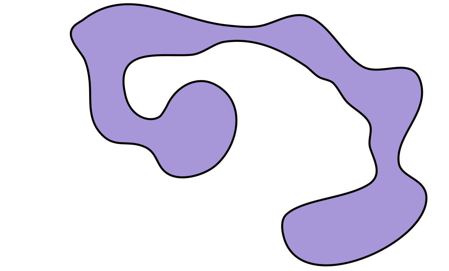
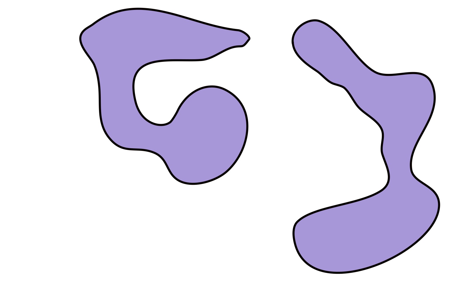
In general, our position will be that we can recognize path-connectedness when we see it. For example, consider the sets in $\R^2$:

drawing

The set above is path-connected, while the set below is not.

drawing

Because we can determine whether a set is path-connected by looking at it, we will not often go to the trouble of giving a rigorous mathematical proof of path-conectedness. If we decide to prove it, then the main point of the proof will be to write down in mathematical language an argument that captures our geometric intuition. Here are a couple of examples:

Example 1.

A ball $B(\mathbf a; r)$ is path-connected.

Our geometric intuition: If $\mathbf x, \mathbf y$ both belong to $B(\mathbf a; r)$, then by drawing a picture, we are confident that the straight line segment that starts at $\mathbf x$ and ends at $\mathbf y$ is a continuous path joining $\mathbf x$ to $\mathbf y$, which stays inside $B(\mathbf a; r)$.

Formal proof

We can write down the above idea using mathematical language. The “straight line segment that starts at $\mathbf x$ and ends at $\mathbf y$” is $\gamma(t)=\mathbf x + t(\mathbf y - \mathbf x)$.
We have to check 3 things:

$\gamma : [0,1]\to B(\mathbf a; r)$ is continuous — which it is, since it is a polynomial
$\gamma(0)=\mathbf x$ and $\gamma(1) = \mathbf y$ — also true, by checking
$\gamma(t)\in B(\mathbf a; r)$ for all $t\in [0,1]$. In other words, we have to show that \[|\gamma(t) - \mathbf a|<r \text{ for all } t\in [0,1].\]

The third condition is not obvious, but our geometric idea is very convincing, so we can be confident that it’s actually true. Like many inequalities coming from pictures of straight lines, we will use the triangle inequality. \[\begin{align*} |\gamma(t) - \mathbf a| &= |(1-t) \mathbf x + t\mathbf y - \mathbf a| &\text{definiton of $\gamma(t)$}\\\ &= |(1-t) (\mathbf x-\mathbf a) + t(\mathbf y - \mathbf a)| &\text{rewrite}\\\ &\le |(1-t) (\mathbf x-\mathbf a)| + |t(\mathbf y - \mathbf a)| &\text{triangle ineq.}\\\ %&= %|1-t|\, |\mathbf x-\mathbf a| + |t|\ |\mathbf y - \mathbf a| &\text{triangle ineq.}\\\ &< (1-t) r + t r = r &\text{ since $\mathbf x, \mathbf y \in B(\mathbf a; r)$}. \end{align*}\] Thus $B(\mathbf a; r)$ satisfies condition $\eqref{pc1}$, and hence it is path-connected.

Remark. The formula $\mathbf x+t(\mathbf y -\mathbf x)$ for a path corresponding to the line segment that starts at $\mathbf x$ and ends at $\mathbf y$ appears very frequently in mathematics, and should be committed to memory. You might recognize it from MAT 223 as describing the set of convex linear combinations of the vectors $\mathbf x$ and $\mathbf y$.

Example 2.

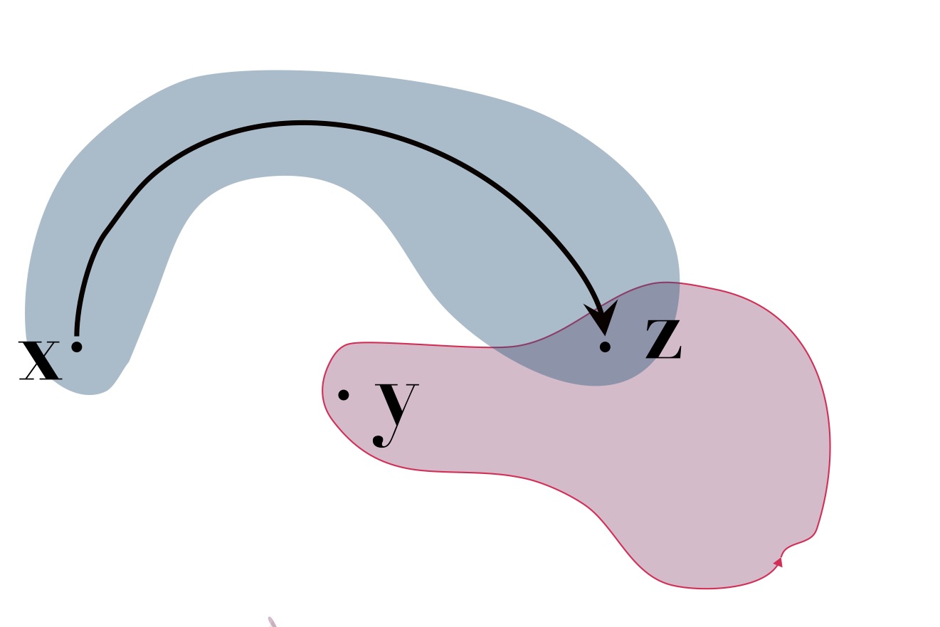
If $S_1$ and $S_2$ are path-connected, and $S_1\cap S_2 \ne \emptyset$, then $S = S_1\cup S_2$ is path-connected.

Our geometric intuition: Consider any $\mathbf x$ and $\mathbf y$ in $S$. If they are both in $S_1$ or $S_2$, then we have a path connecting them, so we are only interested in the case where they are in different sets. Suppose without loss of generality that $\mathbf x \in S_1$ and $\mathbf y \in S_2$.

drawing

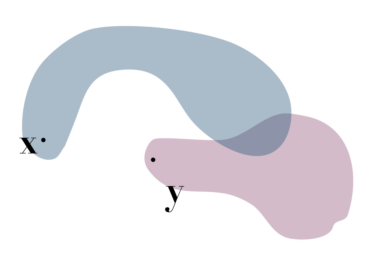
To find a path connecting these two points, let $\mathbf z$ be an element of $S_1\cap S_2$.

drawing

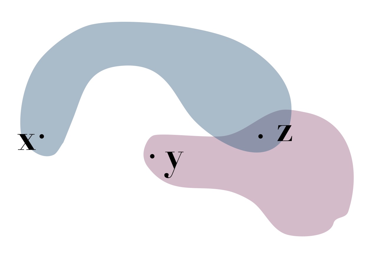
Then since $\mathbf z$ and $\mathbf x$ both belong to $S_1$, we can find a continuous path connecting $\mathbf x$ to $\mathbf z$ that stays in $S_1$, and hence in $S$.

drawing

Similarly, we can find a continuous path connecting $\mathbf z$ to $\mathbf y$ that stays in $S_2$.

drawing

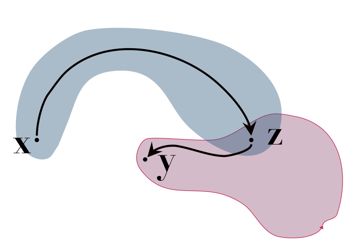
Now we can move continuously from $\mathbf x$ to $\mathbf y$, while staying inside $S$, by concatenating the paths, i.e. first following the continuous path from $\mathbf x$ to $\mathbf z$; then following the continuous path from $\mathbf z$ to $\mathbf y$.

drawing

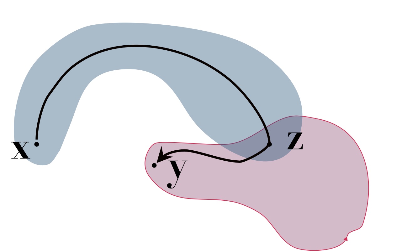
In this way, we can find a path conecting any two points $\mathbf x$ and $\mathbf y$.

Formal proof

We will carefully follow the above geometric intuition. Suppose we are given points $\mathbf x, \mathbf y \in S$. If they are both in $S_1$ or both in $S_2$, then the assumption that each set is path connected gives us a continuous path. So we can assume $\mathbf x \in S_1$ and $\mathbf y \in S_2.$

Fix a point $\mathbf z \in S_1\cap S_2$. Here we are using the hypothesis that $S_1\cap S_2\ne \emptyset$.

Since $\mathbf x$ and $\mathbf z$ both belong to $S_1$, they can be connected by a path, say $\gamma_x$, that stays in $S_1$, and hence inside $S$. That is, \[ \exists \text{ continuous }\gamma_x:[0,1]\to S \text{ such that }\gamma_x(0) = \mathbf x, \text{ and } \gamma_x(1) ={\mathbf z}. \]

By exactly the same reasoning, \[ \exists\text{ continuous }\gamma_y:[0,1]\to S \text{ such that }\gamma_y(0) = {\mathbf z}, \text{ and } \gamma_y(1) ={\mathbf y}. \]

Now we have to figure out how to write down our idea of joining the two paths together to obtain a single continuous function $\gamma:[0,1]\to S$ that starts at $\mathbf x$ and ends at $\mathbf y$. First we patch the two paths together to define $\widetilde \gamma:[0,2]\to S$ by \[\begin{equation}\label{tg} \widetilde \gamma(t) = \begin{cases} \gamma_x(t) &\text{ if }t\in [0,1]\\\ \gamma_y(t-1) &\text{ if }t\in [1,2] \ . \end{cases} \end{equation}\] This satisfies \[ \widetilde \gamma(t) \in S, \qquad \widetilde \gamma(0) = \mathbf x, \qquad \widetilde \gamma(2) = \mathbf y. \]As with other piecewise defined functions, it is continuous because each piece is continuous, and they are both equal to $\mathbf z$ at $t=1$. The only problem is that we want a function with the domain $[0,1]$ instead of $[0,2]$. But this is easy to fix, by defining \[ \gamma(t) = \widetilde \gamma(2t),\qquad t\in [0,1]. \]Then $\gamma$ satisfies $\eqref{pc1}$. Since $\mathbf x$ and $\mathbf y$ were arbitrary points in $S = S_1\cup S_2$, it follows that $S$ is path-connected.

A useful tool for proving subsets are connected is the following theorem, which allows us to build more complicated path-connected sets out of simpler ones using continuous functions:

Suppose that $S\subseteq \R^n$ is path-connected and that $\mathbf f:S\to \R^k$ is continuous. Then the image $\mathbf f(S)\subseteq \R^k$ is also path-connected.

Pick arbitrary points $\mathbf x,\mathbf y\in \mathbf f(S)$. By definition of $\mathbf f(S)$ there exist $\mathbf u,\mathbf v\in S$ such that $\mathbf x = \mathbf f(\mathbf u)$ and $\mathbf y = \mathbf f(\mathbf v)$.

By assumption, $S$ is path-connected so there exists a continuous path $\lambda:[0,1]\to S$ with $\lambda(0)=\mathbf u$ and $\lambda(1)=\mathbf v$. Define $\gamma=\mathbf f\circ\lambda$, ie. the function $\gamma:[0,1]\to \mathbf f(S)$ defined by $\gamma(t)=\mathbf f(\lambda(t))$. This is continuous since it is the composition of continuous functions. Furthermore, $\gamma(0)=\mathbf f(\lambda(0))=\mathbf f(\mathbf u)=\mathbf x$ and similarly $\gamma(1)=\mathbf f(\lambda(1))=\mathbf f(\mathbf v)=\mathbf y$.

Since this shows the existence of a continuous path from $\mathbf x$ to $\mathbf y$ for an arbitrary choice of points $\mathbf x,\mathbf y\in\mathbf f(S)$ we have proven $\mathbf f(S)$ is path-connected.

Example 3.

The set $S=\{(\sin(xyz),x^2-z^2,y-z)\in \R^3 : |(x,y,z)|<1 \}$ is path-connected.

Solution

It is the image of the open ball $B(\mathbf 0; 1)\subseteq \R^3$ via the continuous function $f:\R^3\to \R^3$ with $f(x,y,z)=(\sin(xyz),x^2-z^2,y-z)$.

Example 4.

The graph of any continuous function with path-connected domain is path-connected.

Solution

Let $\mathbf f:S\to \R^k$ be a continuous function with $S\subseteq \R^n$ path-connected. Consider its graph $\mathcal G_{\mathbf f}=\{(\mathbf x,\mathbf f(\mathbf x)): \mathbf x \in S\}.$ Note that $\mathcal G_{\mathbf f}\subseteq \R^{n+k}$. Define ${\mathbf F}:S\to \R^{n+k}$ by ${\mathbf F}(\mathbf x)=(\mathbf x,\mathbf f(\mathbf x))$. This is continuous and $\mathcal G_{\mathbf f}={\mathbf F}(S)$. Thus the graph of $\mathbf f$ is path-connected, since it is the image of the path-connected set $S$ under the continuous function ${\mathbf F}$.

The Intermediate Value Theorem

Having given the definition of path-connected and seen some examples, we now state an $n$-dimensional version of the Intermediate Value Theorem, using a path-connected domain to replace the interval in the hypothesis.

Assume that $S$ is a path-connected subset of $\R^n$ and that $f:S\to \R$ is continuous. If $\mathbf a, \mathbf b$ are points in $S$ and either \[ f(\mathbf a) < t <f(\mathbf b), \qquad \text{ or }\quad f(\mathbf b) < t <f(\mathbf a), \]then there exists a point ${\mathbf c} \in S$ such that $f({\mathbf c})=t$.

Details

Because $S$ is path-connected, there exists a continuous $\gamma:[0,1]\to S$ such that $\gamma(0)=\mathbf a$ and $\gamma(1) = \mathbf b$.

Now define $\phi: [0,1]\to \R$ by $\phi = f\circ \gamma$.

Because both $f$ and $\gamma$ are continuous, we know that $\phi$ is continuous. Also, by hypothesis either \[ \phi(0) = f(\mathbf a) < t <f(\mathbf b)= \phi(1) , \qquad \text{ or }\quad \phi(1) = f(\mathbf b) < t <f(\mathbf a) =\phi(0). \] So the Intermediate Value Theorem for functions of a single variable implies that there exists $s\in [0,1]$ such that $\phi(s) = t$.

But since $\phi(s) = f(\gamma(s))$, if we let ${\mathbf c} = \gamma(s)$, then ${\mathbf c} \in S$ and $f({\mathbf c})=t$.

As with functions of a single variable, the theorem can be used to show that certain equations have solutions. The following example is a little artificial but it illustrates this point.

Example 5.

Prove that the equation \[ x^2+2y^2 = e^{(z-\frac 12)^2 \cos(e^{-\sin (y/(x+2))}) } \] has a solution in the ball $B(\mathbf 0; 2)\subseteq \R^3$.

Solution

To solve this, let’s rewrite the problem as $f(x,y,z)=0$ for $f(x,y,z) = x^2+2y^2 - e^{(z-\frac 12)^2 \cos(e^{-\sin (y/(x+2))})}$. Note that \[f(0,0,\frac 12) = -e^0 = -1<0\] \[f(0,1, 1/2) = 2-e^0 = 1>0.\] Both of these points belong to $B(\mathbf 0; 2)$. We also know that the ball is pathwise connected, so it follows from the Intermediate Value Theorem that there must exist some point in $B(\mathbf 0; 2)$ where $f=0$.

Example 6

Suppose that $S$ is a subset of $\R^n$. The Intermediate Value Theorem implies that if there exists a continuous function $f:S\to \R$, a number $c\in \R$ and points $\mathbf a,\mathbf b\in S$ such that \[ f(\mathbf a)< c, \qquad f(\mathbf b)>c, \qquad f(\mathbf x)\ne c \text{ for any }\mathbf x\in S \]then $S$ is not path-connected.

This can be used to prove that some sets $S$ are not path connected. For example, show that \[ S = \{(x,y)\in \R^2 : x^2 - y^2 \ge 1 \} \]is not path connected.

Solution

Let $f(x,y) = x$, and let $\mathbf a = (-1,0)$ and $\mathbf b= (1,0)$. Then $f(\mathbf a) = -1$ and $f(\mathbf b)=1$. But $S$ cannot contain any points where $f(x,y)=0$, since \[\begin{align*} f(x,y)=0 &\Rightarrow x=0 \\ &\Rightarrow x^2-y^2 = -y^2 \le 0 \\ &\Rightarrow y=0 \end{align*}\]But $(0,0)\not \in S$, so by the Corollary, $S$ is not path-connected.

Problems

Basic

Give examples of a set that is path-connected and one that is not path-connected which have not been discussed in this section.
Let $Q_j\subseteq \R^2$ denote the (open) $j$th quadrant, for $j=1,\ldots, 4$, so that \[\begin{align*} Q_1&= \{(x,y)\in \R^2 : x>0\text{ and }y>0\}, \\ Q_3&= \{(x,y)\in \R^2 : x< 0\text{ and }y< 0\}. \end{align*}\] Determine which of the following sets are path-connected. Formal proofs are unnecessary.
- $Q_1$
- $Q_1\cup Q_3$
- $\overline Q_1 \cup Q_3$
- $\overline Q_1 \cup \overline Q_3$.
- $\partial Q_1\cup Q_3$.
- $\partial( Q_1\cup Q_3)$
Show that the equation $x^2y-y^2z= \cos(xyz)+1$ has a solution on the path-connected set \[S=\left\{\mathbf x \in \R^3: 1<|\mathbf x|<3\right\}.\] See Example 5.

Advanced

Determine whether a set is path-connected, and explain why your answer is correct. Consider for example the same sets appearing in the “Basic Skills” above.
(Recall that in this class, explain means: give a mathematical argument that may fall short of a formal proof but that commnunicates a basic relevant mathematical idea. In this case, to explain why a set is path-connected, you might describe how to connect any two points in a set by a continuous path, without writing down a formula for the path.)
If $S_1$ and $S_2$ are path-connected sets in $\R^2$, must it be true that $S_1\cap S_2$ is path-connected? Explain your answer.
A set $S\subseteq \R^n$ is defined to be star-shaped about the origin if, \[ \forall \, \mathbf x \in S, \forall \lambda\in [0,1] \qquad\text{ the point }\lambda \mathbf x \in S. \]
- Is a ball $B(\mathbf 0; r)$ star-shaped about the origin?
- Draw a picture of a set $S \subseteq\R^2$ that is star-shaped about the origin and that contains the points $(10,0)$ and $(0,10)$, but not the point $(1,1)$.
- Every set that is star-shaped about the origin is path-connected. Give a pictorial argument to explain why this is true.
- Prove that every set that is star-shaped about the origin is path-connected by converting your pictorial argument into a mathematical proof.
Let $S$ denote the unit sphere in $\R^n$: \[ S = \{ \mathbf x \in \R^n : |\mathbf x|=1, \}. \]
- Determine, without proof, whether or not $S$ is path-connected.
- Give a proof to show that your answer is correct.
Let \[ S^+ = \{ \mathbf x = (x_1,\ldots, x_n)\in \R^n : |\mathbf x|=1, \ x_n \ge 0 \}. \] and \[ S^- = \{ \mathbf x = (x_1,\ldots, x_n)\in \R^n : |\mathbf x|=1, \ x_n \le 0 \}. \] One might call these sets the “upper hemisphere” and “lower hemisphere” respectively.
- Draw a picture of $S^+$ when $n=3$.
- Determine (without proof) whether $S^+$ is path-connected.
- If you wish, give a proof to show that your answer to the above question is correct. For this, it may be helpful to write a point $\mathbf x = (x_1,\ldots, x_n)\in S^+$ in the form \[ \mathbf x = (x_1,\ldots, x_{n-1}, f(x_1,\ldots, x_{n-1})) \]where $f(x_1,\ldots, x_{n-1}) =\sqrt{1- (x_1^2 + \cdots + x_{n-1}^2)}.$ Note that $x_1^2 +\ldots + x_{n-1}^2 \le 1$, so the function makes sense.
Let $S$ denote the unit sphere in $\R^n$, as in problem 7, and assume that $f:S\to \R$ is continuous. Prove that there exists some $\mathbf x\in S$ such that $f(\mathbf x) = f(-\mathbf x)$. This implies, for example, that at any given moment, there are two exactly antipodal points on the earth where the temperature is exactly the same.

Hint

Consider the function $g(\mathbf x) = f(\mathbf x) - f(-\mathbf x)$. If you have done problem 7, you know that $S$ is pathwise connected. Use this in your solution.

$\Leftarrow$ $\Uparrow$ $\Rightarrow$

This work is licensed under a Creative Commons Attribution-NonCommercial-ShareAlike 2.0 Canada License.