\(\renewcommand{\R}{\mathbb R }\)
\(\Leftarrow\) \(\Uparrow\) \(\Rightarrow\)
There are two common ways to picture a function \(f:\R^2\to \R\):
By its graph, that is, \[ \{ (x,y,z)\in \R^3 : z = f(x,y)\} \]This is a two-dimensional surface in a \(3\)-dimensional space, whose “height” \(z\) over the \(xy\)-plane at a point \((x,y)\) is the value \(f(x,y)\) of the function at that point. Some examples can be found below.
By its level curves:
We then plot a few different level curves in the \(xy\)-plane, corresponding to different values of \(c\) in the range of \(f\). These values of \(c\) are usually chosen to be evenly spaced, for example \(c = -1, 0, 1, \ldots, 5\). The distance between adjacent curves near a point provides useful information about the rate of change of the function near that point. Curves that are close together mean the function changes rapidly in that region of the plane.
Sketching graphs or level curves by hand both require a lot of practice. The advantage of level curves over graphs is that you already have a lot of practice drawing curves in \(\R^2\), but you probably don’t have much practice drawing surfaces in \(\R^3\). Here are some computer generated images of paraboloids, one elliptic (level curves are ellipses) and one hyperbolic (level curves are hyperbolas):
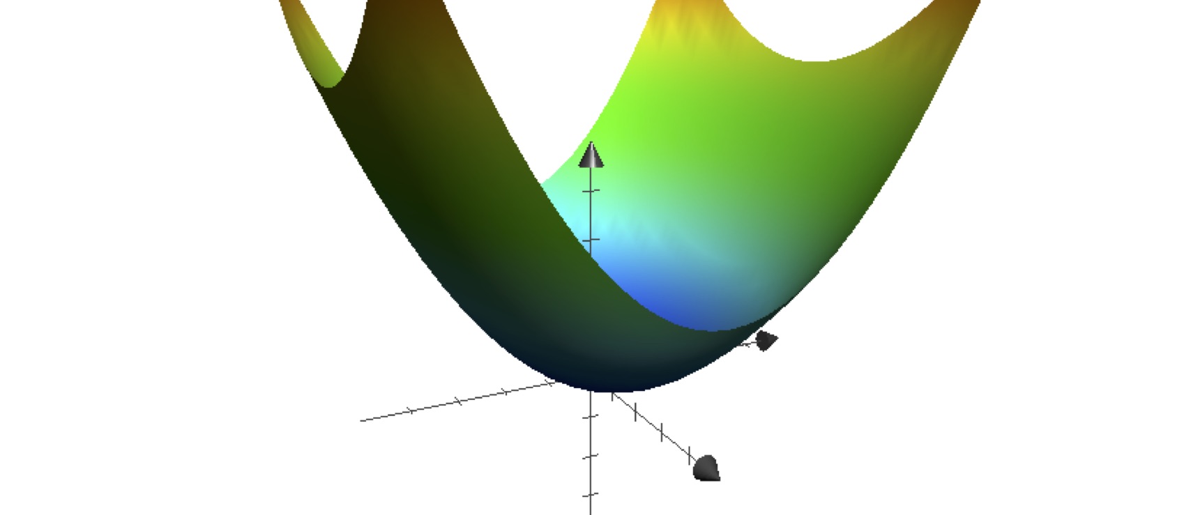
above: graph of the function \(f(x,y)= \frac 19 x^2 + \frac 14 y^2\)
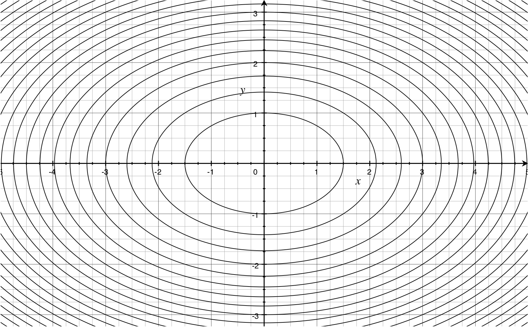
above: level curves of the same function
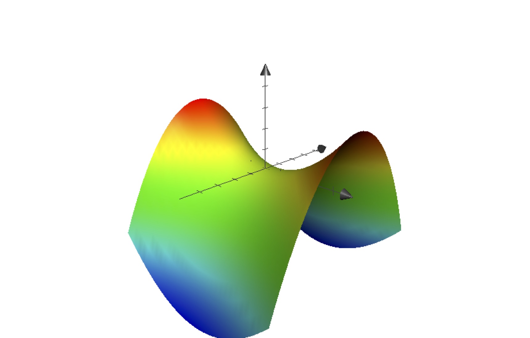
above: graph of the function \(f(x,y) = \frac 19 x^2 - \frac 14 y^2\).
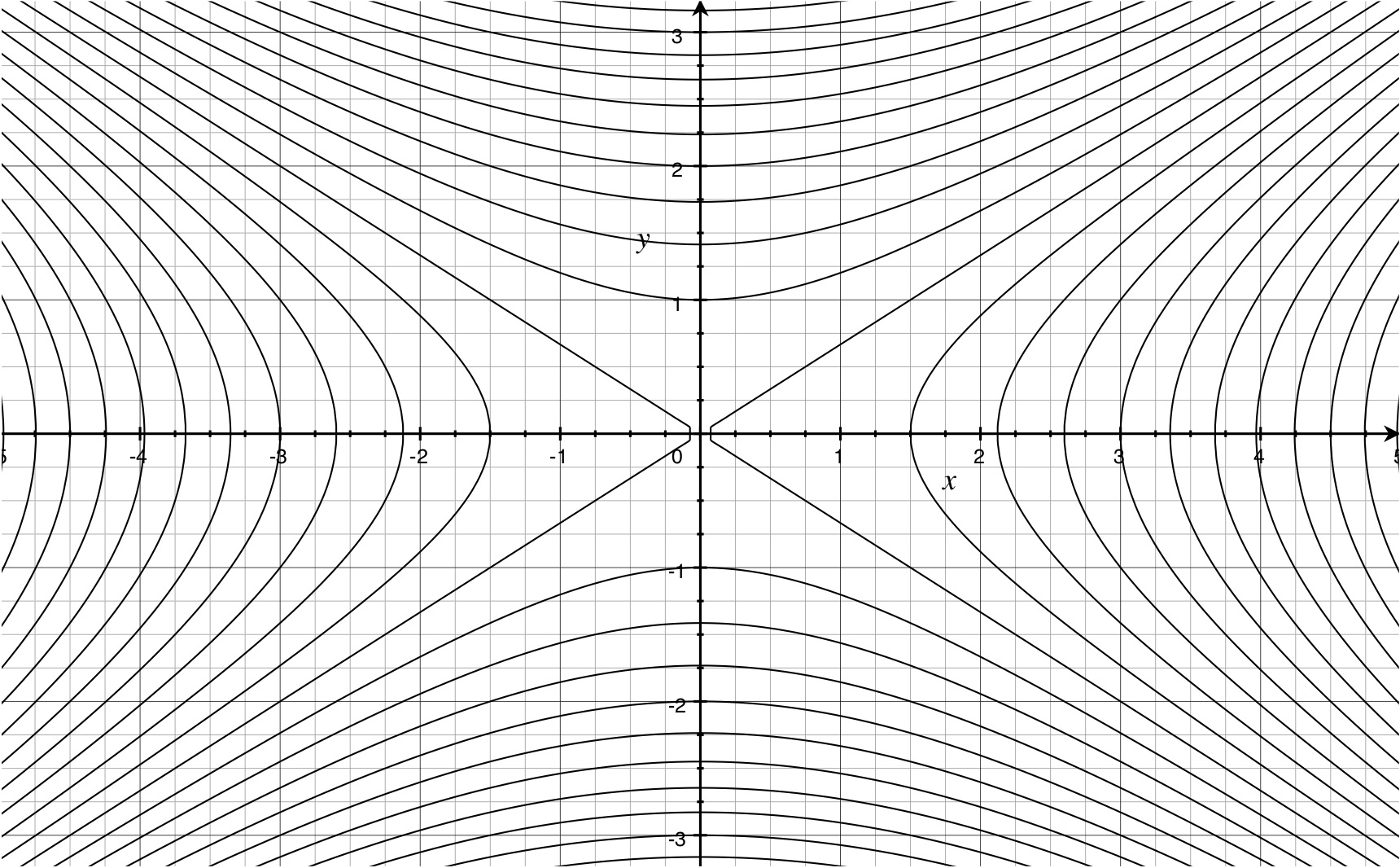
above: level curves of the same function.
You can generate graphs of functions using a SageMathCell. Once it has rendered, you can rotate and zoom to get different perspectives.
You can change anything in the cell and evaluate again. For example, draw the elliptic paraboloid above by changing \(-\) to \(+\). Sage is very particular about algebraic operations, for example, you need to write \(\texttt{2*y}\) instead of \(\texttt{2y}\). Plot more complicated functions, like
If you would like the graph coloured by height, include \(\texttt{adaptive=True, color=rainbow(60, 'rgbtuple')}\) in the plot3d options. This will make it take longer to render. For more options, evaluate \(\texttt{plot3d?}\) or read the Sage reference.
To draw level sets, use the contour_plot class. For more options, evaluate \(\texttt{contour_plot?}\) or read the Sage reference.
Finally, a contour plot of the complicated function above:
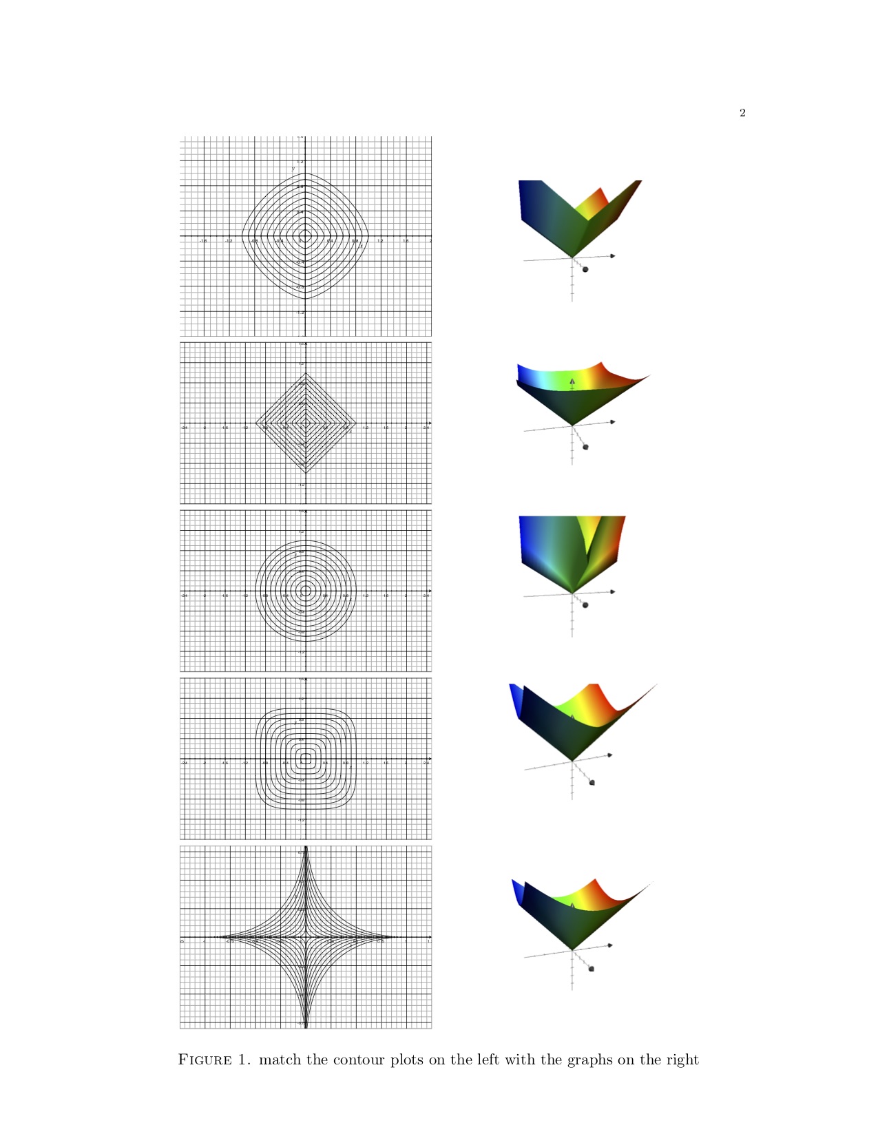
We will not ask you to draw graphs of functions of two variables, and we will rarely ask you to plot level curves. But you will be able to look at one of the pictures and understand what the other would look like, and hence how the function “looks”. One way to practice this skill is to match graphs with level curves. Try it in the images below.
For a function \(f:\R^3\to \R\), we can still define the graph \[ \{ (x, y, z, w) \in \R^4 : w = f(x,y,z) \} \] For most humans, however, it is very hard to form a mental picture of this object, which is a \(3\)-dimensional shape sitting inside a \(4\)-dimensional space.
We can also still define the analog of level sets of a function \(f:\R^3\to \R\). These are sets of the form \(\{ (x,y,z)\in \R^3 : f(x,y,z) = c \}\) for different choices of \(c\). They are sometimes called “level surfaces” to distinguish them from the lower dimensional version. Just like in \(2\) dimensions, these are easier to visualize than the graph. Here are some examples:
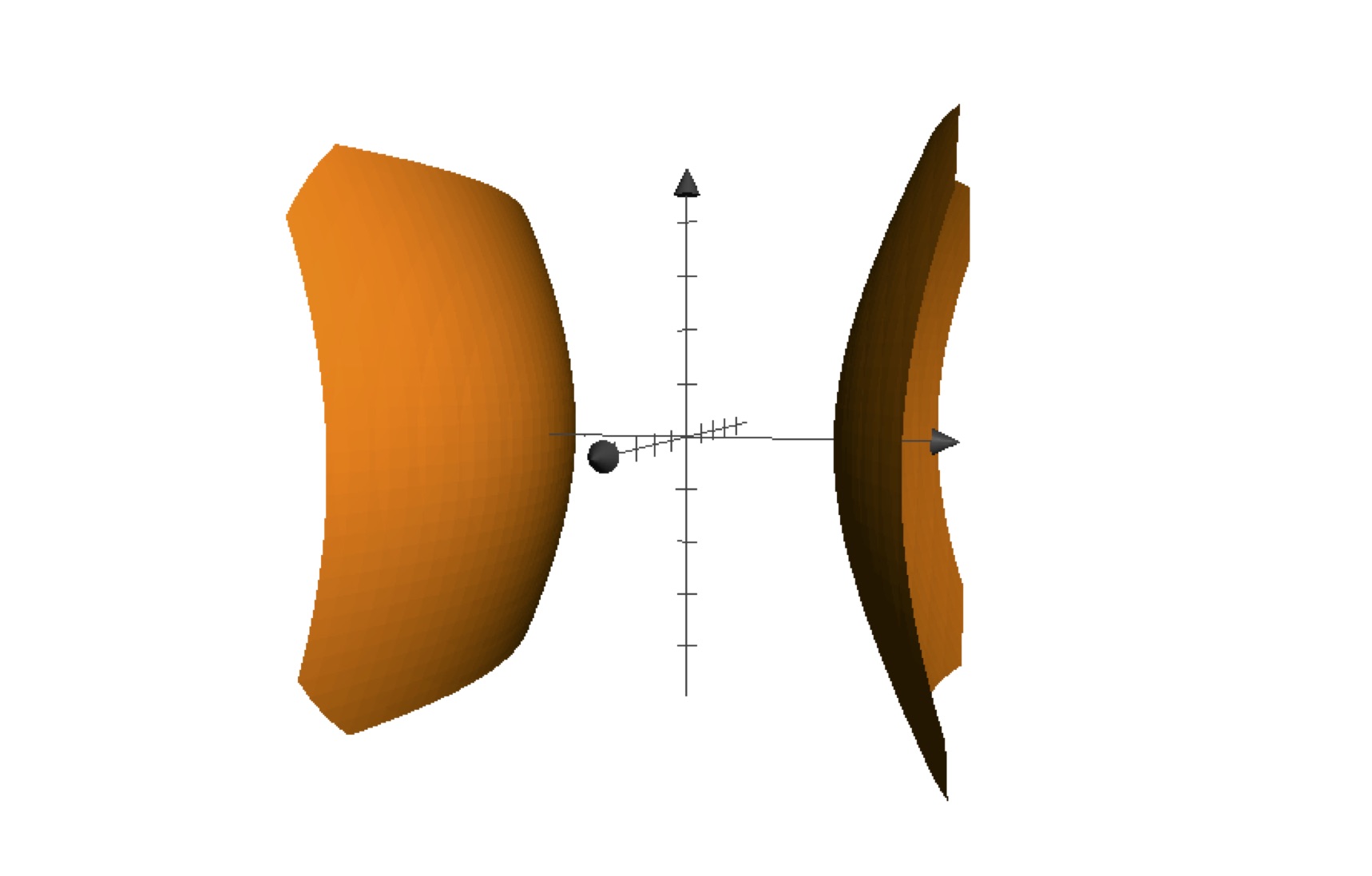
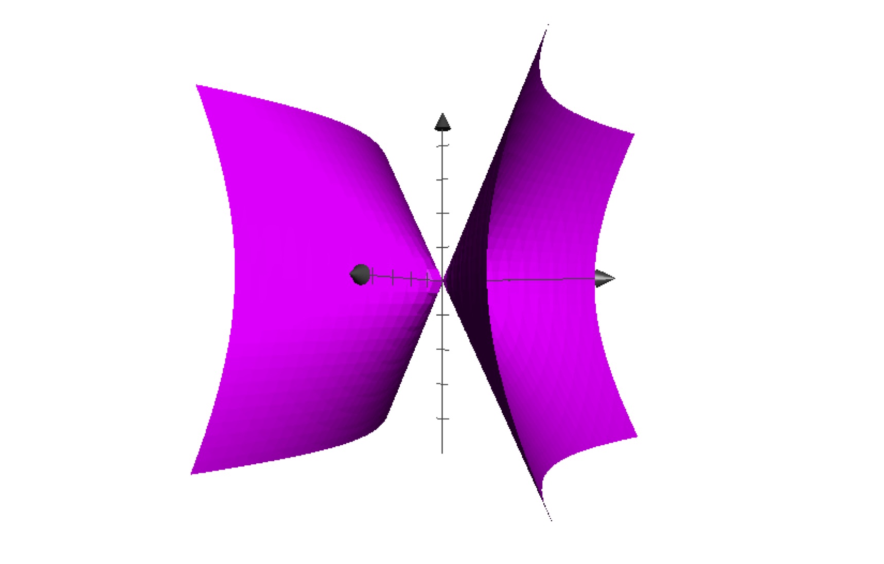
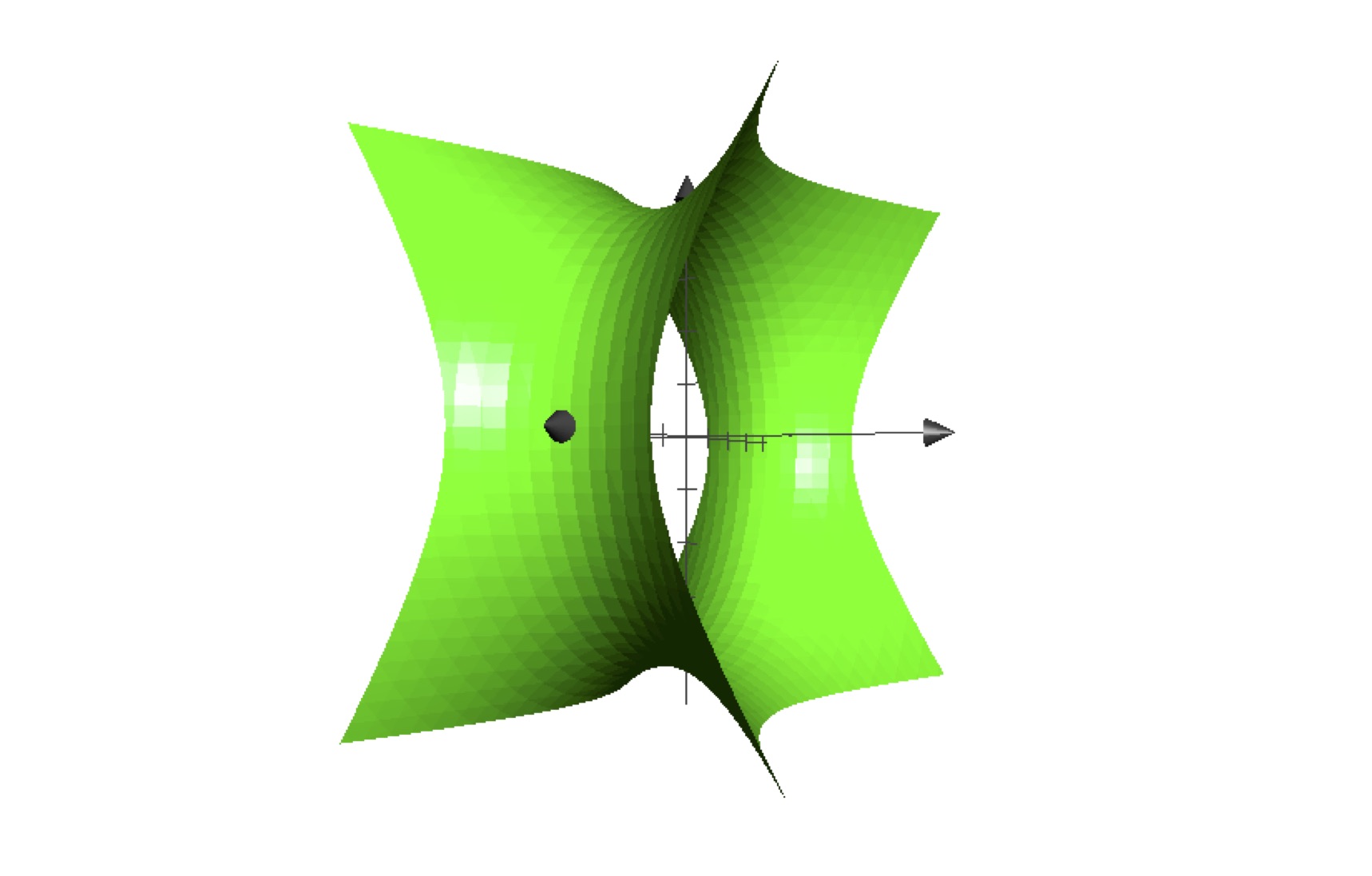
Above: for \(f(x,y,z)= \frac 19 x^2 - \frac 14 y^2 + \frac 19 z^2\), the level surfaces corresponding to \(c=-2, 0, 2\) (from top to bottom).
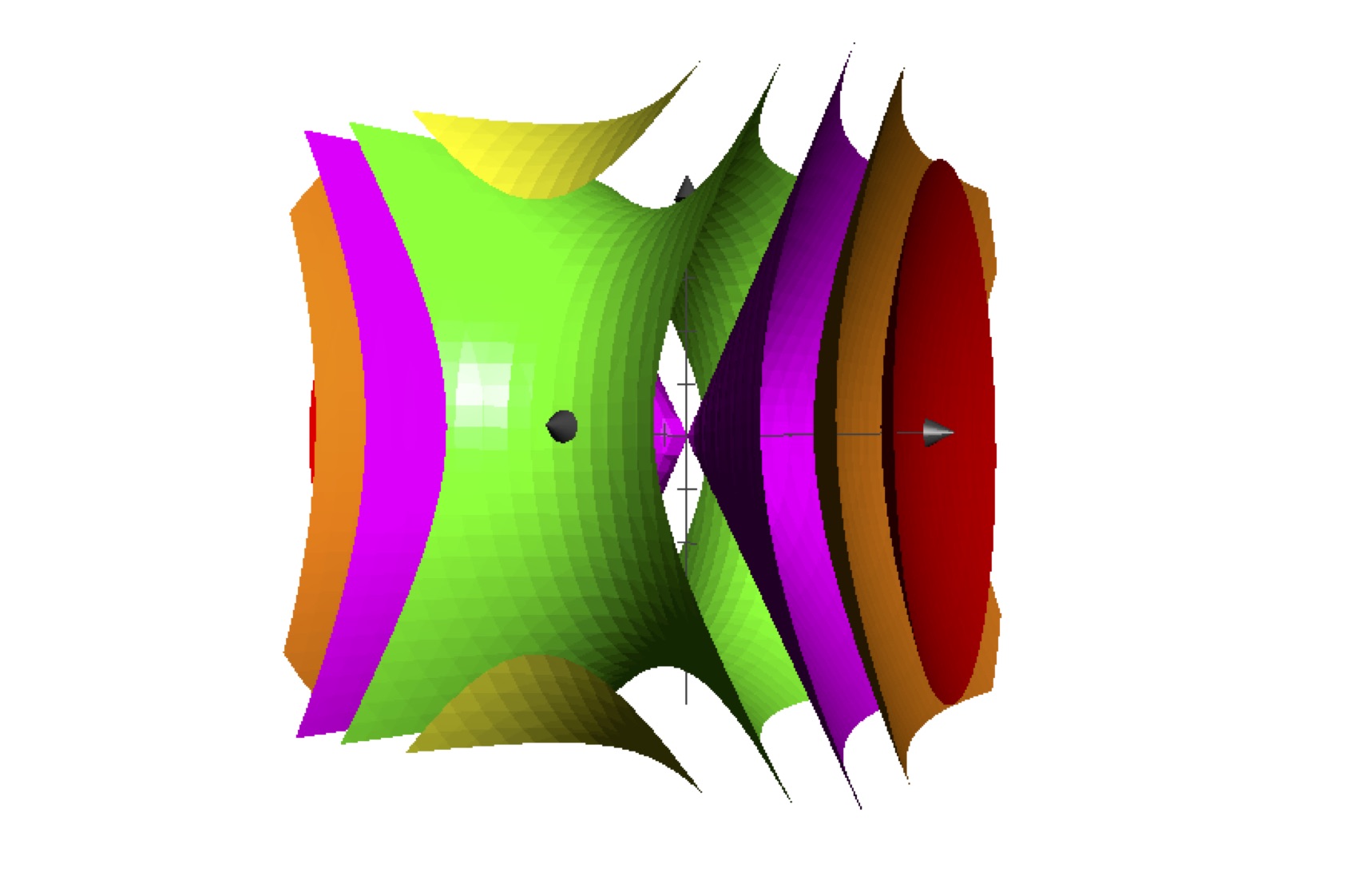
One can also assemble a number of level surfaces into a single image. Here are several level surfaces of \(f(x,y,z)= \frac 19 x^2 - \frac 14 y^2 + \frac 19 z^2\).
Sometimes the level surfaces can be written in the form \(z=f(x,y)-c\), and you can picture them as shifted graphs of a function of two variables. This situation is the simplest possible, so it may help you visualize what happens in higher dimensions, but it is rare.
For functions \(f:\R^n\to \R\), we can define the graph \[ \{ (x_1,\ldots, x_{n+1}) \in \R^{n+1} : x_{n+1} = f(x_1,\ldots, x_n) \} \]and the level sets \[ \{ (x_1,\ldots, x_{n}) \in \R^{n} :f(x_1,\ldots, x_n) = c \} \]but it is very hard to draw an accurate picture or to form a good mental image of either of these, when \(n\ge 4\).
\(\Leftarrow\) \(\Uparrow\) \(\Rightarrow\)

This work is licensed under a Creative Commons Attribution-NonCommercial-ShareAlike 2.0 Canada License.