 |
Dror Bar-Natan Department of Mathematics Princeton University (Currently at the Institute of Mathematics, The Hebrew University, Jerusalem 91904) |
| Dror Bar-Natan: Publications: | 1991 |
| |
Dror Bar-Natan Department of Mathematics Princeton University (Currently at the Institute of Mathematics, The Hebrew University, Jerusalem 91904) |
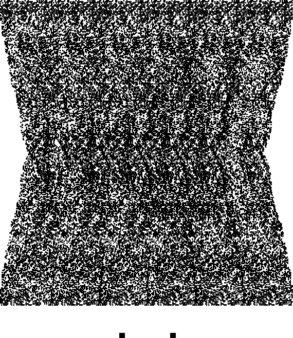
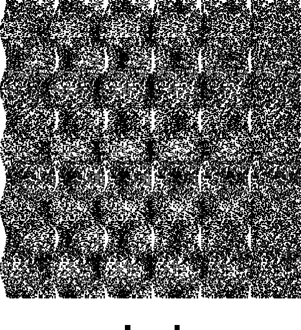
![Sin[r]](Sin_r.gif)
PDIPlot[Sin[Abs[x+I y]],{x,-10,10},{y,-10,10}, PlotPoints -> 120,
  AspectRatio -> Automatic]
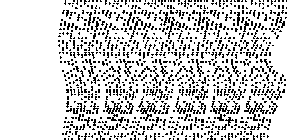
What is this thing? It's a Perceived Depth Image (PDI). It looks like
a random mess, but it isn't. It's a three dimensional plot of the graph of
sin|z|, z=x+iy, in the range
-10<=x,y<=10.
To see it, stare
straight through the page, as if the journal you are holding weren't there,
and let your eyes relax until the two guiding blocks at the bottom of
the figure appear to separate and become four. Focus your eyes at some plane
far behind the figure, and make two of the
four blocks coincide so that you
now see exactly three blocks. Now raise your eyes slowly up to the main
part of the figure, without refocusing them. What you see now is a real,
live, almost touchable, three dimensional picture of sin|z| - a
round valley right at the center, with a circular hill surrounding it, a
circular valley surrounding the hill, ..., all seen from above. Just
the same view could be plotted by
Plot3D[Sin[Abs[x+ I y]],{x,-10,10},{y,-10,10}], only that a PDI
really comes out of the page towards you.
Don't be concerned if you can't see it the first time; it takes some training. Most people need 5-10 minutes to get their first PDI, and after a few more PDI's they can focus at the right distance almost instantaneously. Some people find it easier to start looking at the PDI from about an inch away, and then slowly move the figure away until the image appears. Others find crossing their eyes easier than staring at infinity - you can also view the PDI by holding a pencil in front of the two guiding blocks, focusing your eyes on it, moving it until the two blocks appear to be three, and than looking up the PDI itself.
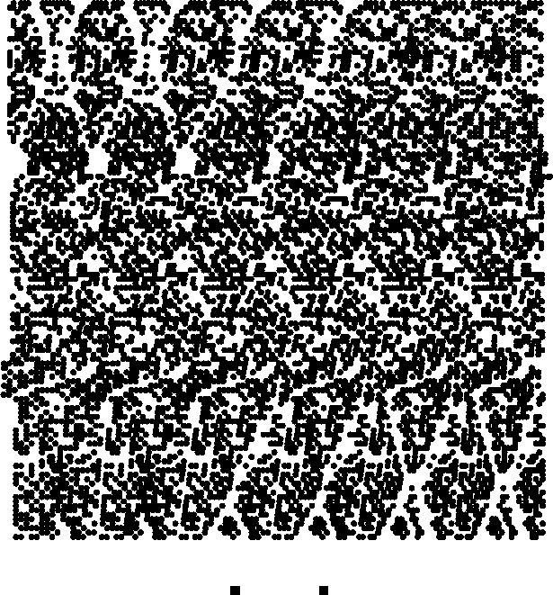
How does it work? Looking more closely at the random mess that makes a PDI, you see that it isn't completely random. Each PDI can be divided into a certain number of vertical strips (6 for the sin|z| picture, for example). The first such strip is randomly filled, the second looks just like the first only a bit distorted, the third is just like the second only distorted some more, and so on. Let us look at a smaller scale example:
SetOptions[PDIPlot,Periods -> 3, PlotPoints -> 12, Guides -> False]
Show[SeedRandom[1]; PDIPlot[0,{x,-1,1},{y,-1,1},
        BasicBlock :> (Line[
          {#1+{1,1}#2,#1+{1,-1}#2,#1+{-1,-1}#2,#1+{-1,1}#2,#1+{1,1}#2}]&)],
     SeedRandom[1]; PDIPlot[2y,{x,-1,1},{y,-1,1},
        BasicBlock :> (Rectangle[#1-.5#2,#1+.5#2]&)],
   AspectRatio -> Automatic]
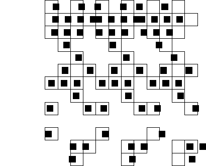
In this example, we first printed a PDI plot of the function 0 (using the
PDIPlot option BasicBlock to make the basic building block of
the picture be an unfilled square), and then,
on top of it, a plot of the function 2y (using smaller blocks). For
clarity, we used the PDIPlot options Periods and
PlotPoints to reduce the resolution of this plot. We also used
the command SeedRandom[1] twice - to make sure that the two
plots would fit neatly one on top of the other. The pattern is now clear
- in the plot of 0, we simply get three identical vertical strips. In the
plot of 2y we can also identify the three vertical strips, but we can see
that they are distorted - the distances between the blocks in the
upper rows, where 2y is positive, are made smaller than the distances
in the lower rows, where 2y is negative.
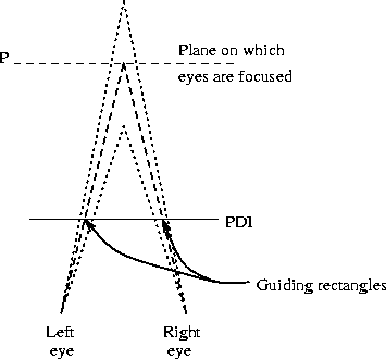
So what? A quick look at figure 1 now explains what happens.
Figure 1: A top view of an observer looking at a PDI.
When we focus our eyes on the plane P, the left eye sees the left guiding block and the right eye sees the right, but our brain interprets it as if there were a single block, on the plane P, and that both our eyes are looking at it. Following now the dotted lines in the figure, it is clear that changing the distance between these two blocks can be interpreted as moving the ``fused'' image block in our brain nearer or farther! A PDI is nothing but a systematic application of this simple phenomenon. See also figure 2.
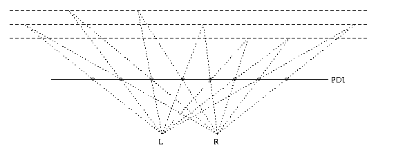
Figure 2: A slightly aperiodic pattern, with the
eyes focused behind the
picture, appears to lie on three different planes. The spaces between
consecutive points relate as 8:9:9:8:7:7:8.
So how do we make a PDI? Well, it's not very hard. A very simple (but crude) code that does a decent job is the following:
z := (-35-30I+x+I y)/30 ; f = Abs[z]*Sin[5Arg[z]]
Show[Graphics[Table[
  xsample=Join @@ Position[Table[Random[]<0.5,{10}],True];
  xv=Outer[Plus,Table[i,{i,0,50,10}],xsample-1];
  xv=xv-Accumulate[Plus,Map[(f /. {y->yi,x->#})&,xv,{2}]];
  Point[{#,yi}]& /@ Flatten[xv],
{yi,60}]]]
The first line is the definition of the expression to be plotted -
essentially it's |z|sin arg z, only with the variables
scaled and shifted a bit. Then comes the main loop - the PDI is
plotted row by row, and yi, that goes from 1 to 60, is
the current value of y. Each row is made of six repetitions of
the same pattern, each distorted by a little relative to the previous
one. The first line of the loop defines xsample to be a
random subset of the integers 1-10. These are the x coordinates
of the pixels that will be turned on in this row of the left most
strip. Then xv is defined to be a list of six copies of
xsample, each shifted by a different amount to form the
current row of the six strips. The next line is the main computation
- the function f is evaluated at each of the points of
xv, and each point x0 in xv
is then shifted, left or right, by the sum of the values of f
on the images of x0 in the strips to its left. This
simply means that the distance between x0 and the
point corresponding to it on the next strip to the left is changed by
f(x0,y) - so when these two points are matched by
the observer's eye, f(x0,y) becomes the depths of the
resulting image point. The last line of the loop just plots the results
of the computation in the line before.
Mandelbrot[c_?NumberQ,n_:32]:=Block[{d,z},
  For[z=0.; d=0, Abs[z]<2 && d<n, d++, z=z^2+c]; d]
PDIPlot[Log[2,Mandelbrot[x+I y]],{x,-2.,1.},{y,-1.5,1.5},
  PlotRange -> {-5,5}, PlotPoints -> 300, BasicBlock -> (Point[#1]&),
  ApparentDepth -> 1.5, AspectRatio -> Automatic, Prolog -> {PointSize[.004]}]
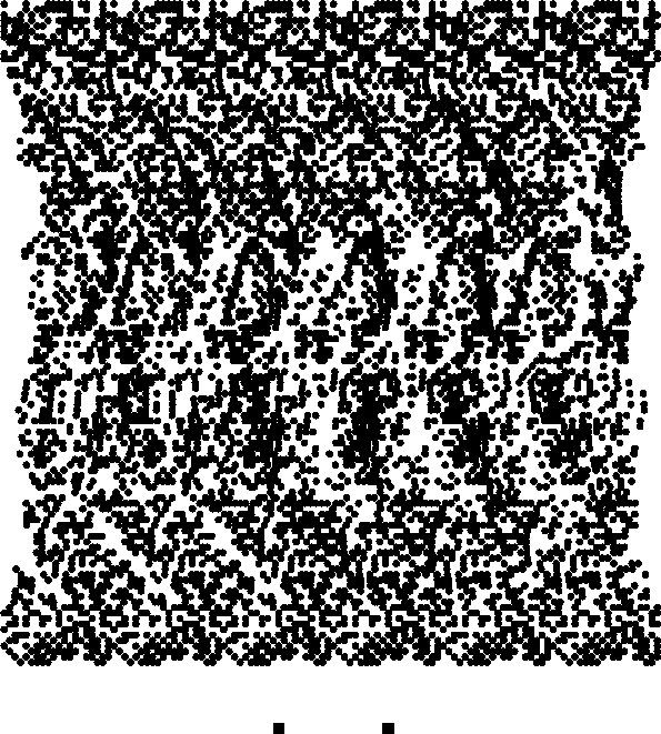
PDIPlot[Abs[x+I y]Arg[(x+I y)^8]/5,{x,-1,1},{y,-1,1}, PlotPoints -> 120,
  BasicBlock -> (Point[#1]&), AspectRatio -> Automatic,
  Prolog -> {PointSize[.01]}]
TorusKnot[m_Integer,n_Integer,z_?NumberQ]:=
  If[z==0,0,
    Block[{distance,knottime,width,i},
      width=.25/n^2 // N;
      Max[0,Table[
        knottime=(Arg[z]+2Pi i)m/n;
        distance=(1+.5Sin[knottime]-Abs[z])^2 // N;
        If[distance>width,0,
          N[.6+.5Cos[knottime]+1.5Sqrt[width-distance]]],
      {i,n}]]
    ]];

plot[m_,n_,pts_]:=PDIPlot[TorusKnot[m,n,x+I y],{x,-2,2},{y,-2,2},
  BasicBlock -> (Point[#1]&), Prolog -> {PointSize[1.2/pts]},
  AspectRatio -> Automatic,PlotPoints -> pts]
plot[3,2,120]
pzol[m_,n_,pts_]:=PDIPlot[1-TorusKnot[m,n,x+I y],{x,-2,2},{y,-2,2},
  BasicBlock -> (Point[#1]&), Prolog -> {PointSize[1.2/pts]},
  AspectRatio -> Automatic,PlotPoints -> pts]
pzol[3,2,120]
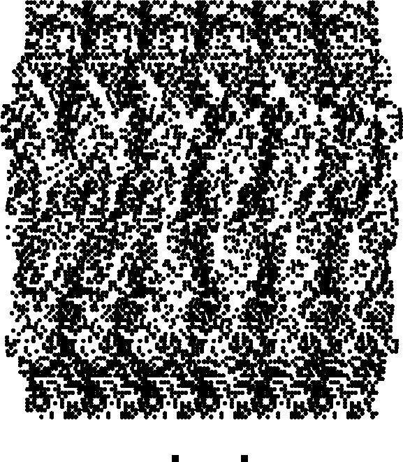
PDIPlot[Cos[x]Cos[y],{x,-15.7,15.7},{y,-15.7,15.7},ApparentDepth->.4,
  BasicBlock->(Point[#1]&),AspectRatio->Automatic,PlotPoints->300,
  Prolog->{PointSize[.004]}]
There are many other directions to check - the
reader is welcome to try to plot other functions, color PDI's,
animated PDI's, .... The reader is advised to first try PDI's of
relatively low resolution (say PlotPoints -> 48 or so), before
attempting to reproduce the PDI's in this article. These were produced on a
fast workstation, and each took few hours of computing time.
PDI.m. The package
PDI.m is just the program displayed before,
with some additional options added. The only substantial
improvement is that a new Graphics primitive,
PDIArray[basicblock_,pts_], is defined. pts
is a list of points, and basicblock is a pure function that
is used to render each point in pts. PDIPlot
gives it's output in the form of a PDIArray, and this
PDIArray is not converted into simpler primitives until
the plot is displayed. This trick saves a significant amount of memory.
For a primitive but working 9 line version of that package, click here.
BeginPackage["PDI`"]

PDIPlot::usage ="\n
  PDIPlot[exp,{x,xmin,xmax},{y,ymin,ymax}] returns a perceived-depth-image\n
  of the graph of the function given by exp. Options:\n
    PlotPoints (can be an integer or pair of integers; defaults to 60);\n
    Periods (6); PlotRange ({-1,1}); Density (.5); ApparentDepth (1.);\n
    Guides (True); BasicBlock (Rectangle[#1-#2,#1+#2]&).\n
    Other options are passed on to Graphics."

SetAttributes[PDIPlot,HoldFirst];

Options[PDIPlot] := {PlotPoints -> 60, Periods -> 6, Guides -> True,
  PlotRange -> {-1,1}, Density -> .5, ApparentDepth -> 1.,
  BasicBlock :> (Rectangle[#1-#2,#1+#2]&)}

Begin["`private`"]

(* A new Graphics primitive *)
Unprotect[Display]
Display[channel_,graphics_?(!FreeQ[#,PDIArray]&)] :=
  (Display[channel,graphics /.
    (PDIArray[basicblock_,size_,pts_] :>
      (basicblock[#,size]& /@
        (Flatten[Outer[List,First[#],{Last[#]}],1])& /@ pts))];
  graphics)
Protect[Display]

PDIPlot[expr_,{x_Symbol,xmin_?NumberQ,xmax_?NumberQ},
	      {y_Symbol,ymin_?NumberQ,ymax_?NumberQ},opts___] :=
  Block[{plotpts    =(PlotPoints     /. {opts} /. Options[PDIPlot]),
         periods    =(Periods        /. {opts} /. Options[PDIPlot]),
         zrange     =(PlotRange      /. {opts} /. Options[PDIPlot]),
         density    =(Density        /. {opts} /. Options[PDIPlot]),
         depth      =(ApparentDepth  /. {opts} /. Options[PDIPlot]),
         basicblock =(BasicBlock     /. {opts} /. Options[PDIPlot]),
         guides     =(Guides         /. {opts} /. Options[PDIPlot]),
         xres,xpts,xv,xsample,xsteps,xfull,xshift,
         ypts,i,yv,zmin,zmax,zmid,zscale},

(* Some scaling calculations *)
    {zmin,zmax} = zrange ; xres=Floor[xpts/periods];
    zmid = (zmax+zmin)/2 ; zscale = .06depth(xmax-xmin)/(zmax-zmin);
    {xpts,ypts} = If[Length[plotpts]==2,plotpts,{plotpts,plotpts}];
(* The strips *)
    xsteps=xres*Table[i,{i,-.5,periods-1.5}];
(* The main program *)
    Show[Graphics[{PDIArray[basicblock,{(xmax-xmin)/xpts,(ymax-ymin)/ypts}/2,
(* Loop over the values of yv *)
      Table[
(* Filling the current row of the left-most strip randomly *)
        xsample=Flatten[Position[Table[Random[]<density,{xres}],True]];
(* The x values to be used in this row *)
        xv=N[xmin+Outer[Plus,xsteps,xsample-1]*(xmax-xmin)/xpts];
(* Computing the left/right shift of every block *)
        z=N[Map[(expr /. {y->yv,x->#})&,xv,{2}]]-zmid;
        xshift=zscale Accumulate[Plus,z];
(* Final positioning of the blocks *)
        xfull=xv-((#-Last[xshift]/2)& /@ xshift);
        {Flatten[xfull],yv}, {yv,ymin,ymax,(ymax-ymin)/ypts}]],
(* If guides==True, add guiding rectangles *)
      If[guides, (Rectangle @@ #)& /@ Map[
          ({.5xmax+.5xmin,1.1ymin-.1ymax}+{xmax-xmin,ymax-ymin}#/2/periods)&,
          {{{-2.1,-.1},{-1.9,.1}},{{-.1,-.1},{.1,.1}}},{2}], {}]},
      Sequence@@Select[{opts},!MemberQ[First /@ Options[PDIPlot],First[#]]&]
  ]] ]

End[]
EndPackage[]
Exercise Take a second look at the PDI plot of sin|z|. You can see that the second circular hill, the last that can be seen in the picture, is a bit `squarish'. Why is it so? How can it be avoided?
Notes. Our PDI's are a slightly modified version of B. Julesz's `Random-dot stereograms' [2], invented by D. S. Falk, D. R. Brill and D. G. Stork [1, 3]. The TLA PDI was coined by a company, 3D-Hardcopy of Salt Lake City, Utah, which is producing full size PDI posters of exactly the same type as ours. To order, call Jeremy Westover at (503) 345-9359. I wish to thank S. Levy for his advice and editorial help.
This document was generated from a TeX source on November 21, 1998. The generation of this document was assisted by the LaTeX2HTML translator Version 96.1-h (September 30, 1996) Copyright © 1993, 1994, 1995, 1996, Nikos Drakos, Computer Based Learning Unit, University of Leeds.
On March 24, 1999, I got the image below from John Sullivan, who found it at Andrei Gnepp's, who got it from an unknown source. It serves as a wonderful postscript to this paper:
-------------------------------*---------------*--------------------------------
here gold slim where gold slim where gold slim where gold slim where gold slim w
ly dog camel silly dog camel silly dog camel silly dog camel silly dog camel sil
eird dish goat weird dish goat weird dish goat weird dish goat weird dish goat w
cky bank mile lucky bank mile lucky bank mile lucky bank mile lucky bank mile lu
d stop rook brand stop rook bran stop crook bran stop crook bran stop crook bran
wasting ill ton wasting ill to wasting pill to wasting pill to wasting pill to w
 your host plant your host plan your ghost plan your ghost plan your ghost plan
s time pot stands time pot stand time spot stand time spot stand time spot stand
egg diet please egg diet please egg diet please egg diet please egg diet please
y a hit fool many a hit fool many a hit fool many a hit fool many a hit fool man
junkyard camels junkyard camels junkyard camels junkyard camels junkyard camels
dise fender paradise fender paradise fender paradise fender paradise fender para
ittles bitter skittles bitter skittles bitter skittles bitter skittles bitter sk
y lucky wow! very lucky wow! very lucky wow! very lucky wow! very lucky wow! ver
-------------------------------*---------------*--------------------------------